Chapter 7 SEM
7.1 Structural Equation Modeling
SEM is the broader umbrella from the GLM. With it we are able to do two interesting this:
Fit a latent measurement model (e.g., CFA)
Fit a structural model (e.g,. path analysis)
7.2 Latent variables
A latent variable is assumes to exist but we cannot directly measure (see) it. Sounds like psychological variables!
The reason why items/indicators/measures correlate is assumed to be due to this latent variable. For example, why does Sally like to go to parties, likes to talk a lot, and always tends to be a in a good mood? Maybe it is because her high levels of extraversion ( a latent variable that we cannot directly measure) is causing these tendencies.
Key point: the variable/construct itself is not measurable, but the manifestations caused by the variable are measurable/observable.
Interesting point: because variables are assumed to be causing indicators of the variable, SEM is sometimes referred to as causal modeling. (Also because in path models a directional relationship is hypothesized) Note that we cannot get any closer to causality than we can with regression.
7.2.1 More pretty pictures
Circles = latent variables
Boxes = observed indicator variables
two headed arrows = correlations/covariances/variances
single head arrows = regressions
triangle = means
7.2.2 Classical test theory interpretation
How can we think of a latent construct:
Latent construct = what the indicators share in common
The indicators represent the sum of True Score variance + Item specific variance + Random error
The variance of the latent variable represents the amount of common information in the latent variable
The residual errors (sometimes referred to as disturbances) represent the amount of information unique to each indicator. A combination of error and item-specific variance.
7.2.3 Generizability interpretation of latent variables
Same as above, but…
True score variance can be thought of as consisting as a combination of 1. Construct variance- this is the truest true score variance 2. Method variance- see Campbell and Fiske or sludge factor of Meehl. 3. Occasion- important for longitudinal, aging, and cohort analyses–and for this class.
For longitudinal models, occasion specific variance can lead to biased estimates. We want to separate the time specific variance from the overall construct variance. Or, we want to make sure that the time specific variance doesn’t make it appear that a construct is changing when really it is not.
7.2.3.1 Formative indicators
These pretty pictures imply that the latent variables “cause” the indicators. These are referred to as reflexive indicators and are the standard way of creating latent variables. However, there is another approach, formative indicators, were indicators “cause” the latent variable. Or, in other words, the latent variable doesn’t actually exist. It is not real, only a combination of variables. An example of this is SES.
7.2.4 measurement error
A major advantage is that each latent variable does not contain measurement error. It is as is if we measured our variable with an alpha = 1.
What does that do? Well, ideally that gets us closer to the population model, which could yield higher R2 and parameter estimates.
How does this happen? It is a direct result of capturing what is shared among the indicators. The measurement error associated with each indicator is uncorrelated with the latent variable.
Think about how this situation differs from creating a composite among variables. Think about how this differs from creating a factor score among variables within a simple factor analyses approach. How are all three different and similar?
What does it mean if the error variances are correlated with one another?
7.2.5 regarding means
SEM is also known as covariance structure analysis. You can do SEM using only variance-covariance matrices. These do not necessarily involve any direct information about their means. Means in SEM are optional.
More later on how we define the mean of a latent variable if we do not assess the mean of the variable in the first place
7.3 goal of SEM
Creation of a model that specifies a certain relationship among variables. This is done by creating a measurement or path model that we think is driven by the data generating process we are trying to study. In addition to setting the measurement model and paths we may want to put apriori constraining parameters (variances/covarainces/regressions) to reflect how we think variables are related.
E.g., Should these two variables be correlated or not?
Then we use or ML algorithm to get our model implied covariances/means as close as possible to the observed covariances/means.
E.g., we specified no correlation between these two variables, does that then change how their indicators relate to their latent variable?
7.3.1 What questions can be asked?
Too many to mention. This is a really flexible approach to your data. Might as well always think about problems in terms of SEM because is subsumes regression models.
Specifically, however, SEM can handle any time of measured DV/IV or construct/indicators.
If you have categorical indicators you can do SEM. However, it is hard to measure change using categorical indicators. But, categorical indicators are used for many latent variable models such as in measuring psychopathology.
If you have a categorical construct you can also do SEM. Here it is called latent transition analysis (if you also had categorical indicators) or latent class / latent mixture modeling if you had continuous indicators (i am counting ordinal as continuous).
7.4 Setting the scale and defining variables
We are trying to measure clouds. How can we do this given that they are always moving?
Need to define a parameter a latent variable because there is no inherent scale of measurement.
Largely irrelevant as to what scale is chosen. Serves to establish a point of reference in interpret other parameters.
3 options:
Fixed factor. Here you fix the variance of the latent variable to 1 (standardized)
Marker variable. Here you fix one factor loading to 1. All other loadings are relative to this loading.
Effect coding. Here you constrain loading to average to 1. This will be helpful for us as we can then put the scale of measurement into our original metric. For longitudinal models this is helpful in terms of how to interpret the amount of change.
7.4.1 identification
All of this works only if you have enough data to be able to create new constructs. As a rule of thumb you need at least three indicators for each latent variable.
More specifically, you need to compare the number of knows (variances and covariances) to the unknowns (model parameters).
Foe example, a three indicator latent variable has 7 unknowns. 3 Loadings, 3 error variances and the variance of the latent variable
The covariance matrix has 6 data points. Thus we need to add in one more known, in this case a fixed factor or a marker variable.
7.4.2 types of identification
just identified is where the number of knowns equal unknowns. also known as saturated model.
over identified is when you have more knowns than unknowns (this is good)
under identified is when you have problems and have more unknowns than knowns. this is because there is more than one solution available and the algorithm cannot decide e.g,. 2 + X = Y. If we add a constraint or a known value then it becomes manageable 2 + X = 12
7.4.2.1 degrees of freedom
knowns - unknowns = df
Note that df in this case will not directly relate to sample size
7.5 lavaan
Easy to use SEM program in R
library(lavaan)## This is lavaan 0.5-23.1097## lavaan is BETA software! Please report any bugs.##
## Attaching package: 'lavaan'## The following object is masked from 'package:psych':
##
## cor2covDoes most of what other sem packages do and just as well except for:
- Multilevel SEM
- Latent class models/mixture models
Two useful add on packages are
library(semTools)## ## ################################################################################# This is semTools 0.4-14## All users of R (or SEM) are invited to submit functions or ideas for functions.## #################################################################################
## Attaching package: 'semTools'## The following object is masked from 'package:psych':
##
## skewlibrary(semPlot)A related package that uses similar syntax for Bayesian models is
library(blavaan)## Loading required package: runjags##
## Attaching package: 'runjags'## The following object is masked from 'package:tidyr':
##
## extract## This is blavaan 0.2-4## blavaan is more BETA than lavaan!7.5.1 lavaan language
All you need to know (almost) is here: http://lavaan.ugent.be/tutorial/
A quick recap of that:
- Paths between variables is the same as our linear model syntax
y ~ x1 + x2 + x3~ can be read as “is regressed on”
- defining latent variables
y =~ x1 + x2 + x3=~ can be read as “measured by”
Y is measured by the variables x1 - x3. This will define the factor loadings.
- defining variances and covariances
y ~~ x1 Y covaries with X1.
The beautify of lavaan is that it will decide for you if you are interested in a variance or a covariance or a residual (co)variance.
- intercept
y ~ 1 Much as we saw with our lmer models where 1 served an important role, 1 here also is special in that it references the mean (intercept) of the variable. This will come in handy when we want to constrain or make the means of variables similar to one another.
- constraints
y =~ NA*x1 + 1*x2 + a*x3 + a*x4NA serves to free a lavaan imposed constraint. Here, the default is to set the first factor loading to 1 to define the latent variable. NA* serves to say there is no constraint.
1* pre-multiples the loading by a particular number. In this case it is 1, to define the latent variable, but it could be any number. R doesn’t know if it makes sense or not.
a* (or and other character strings) serves as an equality constraint by estimating the same parameter for each term with that label. In this case x3 and x4 will have the same factor loading, referred to as a.
7.5.2 How to run lavaan
- Specify your model
- Fit the model
- Display the summary output
#1. Specify your model

HS.model <- ' visual  =~ x1 + x2 + x3
              textual =~ x4 + x5 + x6
              speed   =~ x7 + x8 + x9 '

#2. Fit the model

fit <- cfa(HS.model, data=HolzingerSwineford1939)

  # other functions include sem, growth, and lavaan. All have different defaults (See below). we will use growth a lot.


#3. Display the summary output

summary(fit, fit.measures=TRUE)
7.5.3 lavaan defaults
First, by default, the factor loading of the first indicator of a latent variable is fixed to 1, thereby fixing the scale of the latent variable. Second, residual variances are added automatically. And third, all exogenous latent variables are correlated by default.
lets work with a dataset from the lavaan package
HolzingerSwineford1939 <- HolzingerSwineford1939

mod.1 <- 'visual =~ x1 + x2 + x3
textual =~ x4 + x5 + x6
speed =~ x7 + x8 + x9'

fit.1 <- cfa(mod.1, data=HolzingerSwineford1939)

summary(fit.1, fit.measures=TRUE, standardized=TRUE)
## lavaan (0.5-23.1097) converged normally after 35 iterations
##
## Number of observations 301
##
## Estimator ML
## Minimum Function Test Statistic 85.306
## Degrees of freedom 24
## P-value (Chi-square) 0.000
##
## Model test baseline model:
##
## Minimum Function Test Statistic 918.852
## Degrees of freedom 36
## P-value 0.000
##
## User model versus baseline model:
##
## Comparative Fit Index (CFI) 0.931
## Tucker-Lewis Index (TLI) 0.896
##
## Loglikelihood and Information Criteria:
##
## Loglikelihood user model (H0) -3737.745
## Loglikelihood unrestricted model (H1) -3695.092
##
## Number of free parameters 21
## Akaike (AIC) 7517.490
## Bayesian (BIC) 7595.339
## Sample-size adjusted Bayesian (BIC) 7528.739
##
## Root Mean Square Error of Approximation:
##
## RMSEA 0.092
## 90 Percent Confidence Interval 0.071 0.114
## P-value RMSEA <= 0.05 0.001
##
## Standardized Root Mean Square Residual:
##
## SRMR 0.065
##
## Parameter Estimates:
##
## Information Expected
## Standard Errors Standard
##
## Latent Variables:
## Estimate Std.Err z-value P(>|z|) Std.lv Std.all
## visual =~
## x1 1.000 0.900 0.772
## x2 0.554 0.100 5.554 0.000 0.498 0.424
## x3 0.729 0.109 6.685 0.000 0.656 0.581
## textual =~
## x4 1.000 0.990 0.852
## x5 1.113 0.065 17.014 0.000 1.102 0.855
## x6 0.926 0.055 16.703 0.000 0.917 0.838
## speed =~
## x7 1.000 0.619 0.570
## x8 1.180 0.165 7.152 0.000 0.731 0.723
## x9 1.082 0.151 7.155 0.000 0.670 0.665
##
## Covariances:
## Estimate Std.Err z-value P(>|z|) Std.lv Std.all
## visual ~~
## textual 0.408 0.074 5.552 0.000 0.459 0.459
## speed 0.262 0.056 4.660 0.000 0.471 0.471
## textual ~~
## speed 0.173 0.049 3.518 0.000 0.283 0.283
##
## Variances:
## Estimate Std.Err z-value P(>|z|) Std.lv Std.all
## .x1 0.549 0.114 4.833 0.000 0.549 0.404
## .x2 1.134 0.102 11.146 0.000 1.134 0.821
## .x3 0.844 0.091 9.317 0.000 0.844 0.662
## .x4 0.371 0.048 7.779 0.000 0.371 0.275
## .x5 0.446 0.058 7.642 0.000 0.446 0.269
## .x6 0.356 0.043 8.277 0.000 0.356 0.298
## .x7 0.799 0.081 9.823 0.000 0.799 0.676
## .x8 0.488 0.074 6.573 0.000 0.488 0.477
## .x9 0.566 0.071 8.003 0.000 0.566 0.558
## visual 0.809 0.145 5.564 0.000 1.000 1.000
## textual 0.979 0.112 8.737 0.000 1.000 1.000
## speed 0.384 0.086 4.451 0.000 1.000 1.000Lets use a fixed factor approach rather than a marker variable approach
mod.2 <- 'visual =~ x1 + x2 + x3
textual =~ x4 + x5 + x6
speed =~ x7 + x8 + x9'

fit.2 <- cfa(mod.2, std.lv=TRUE, data=HolzingerSwineford1939)

summary(fit.2, fit.measures=TRUE, standardized=TRUE)
## lavaan (0.5-23.1097) converged normally after 22 iterations
##
## Number of observations 301
##
## Estimator ML
## Minimum Function Test Statistic 85.306
## Degrees of freedom 24
## P-value (Chi-square) 0.000
##
## Model test baseline model:
##
## Minimum Function Test Statistic 918.852
## Degrees of freedom 36
## P-value 0.000
##
## User model versus baseline model:
##
## Comparative Fit Index (CFI) 0.931
## Tucker-Lewis Index (TLI) 0.896
##
## Loglikelihood and Information Criteria:
##
## Loglikelihood user model (H0) -3737.745
## Loglikelihood unrestricted model (H1) -3695.092
##
## Number of free parameters 21
## Akaike (AIC) 7517.490
## Bayesian (BIC) 7595.339
## Sample-size adjusted Bayesian (BIC) 7528.739
##
## Root Mean Square Error of Approximation:
##
## RMSEA 0.092
## 90 Percent Confidence Interval 0.071 0.114
## P-value RMSEA <= 0.05 0.001
##
## Standardized Root Mean Square Residual:
##
## SRMR 0.065
##
## Parameter Estimates:
##
## Information Expected
## Standard Errors Standard
##
## Latent Variables:
## Estimate Std.Err z-value P(>|z|) Std.lv Std.all
## visual =~
## x1 0.900 0.081 11.127 0.000 0.900 0.772
## x2 0.498 0.077 6.429 0.000 0.498 0.424
## x3 0.656 0.074 8.817 0.000 0.656 0.581
## textual =~
## x4 0.990 0.057 17.474 0.000 0.990 0.852
## x5 1.102 0.063 17.576 0.000 1.102 0.855
## x6 0.917 0.054 17.082 0.000 0.917 0.838
## speed =~
## x7 0.619 0.070 8.903 0.000 0.619 0.570
## x8 0.731 0.066 11.090 0.000 0.731 0.723
## x9 0.670 0.065 10.305 0.000 0.670 0.665
##
## Covariances:
## Estimate Std.Err z-value P(>|z|) Std.lv Std.all
## visual ~~
## textual 0.459 0.064 7.189 0.000 0.459 0.459
## speed 0.471 0.073 6.461 0.000 0.471 0.471
## textual ~~
## speed 0.283 0.069 4.117 0.000 0.283 0.283
##
## Variances:
## Estimate Std.Err z-value P(>|z|) Std.lv Std.all
## .x1 0.549 0.114 4.833 0.000 0.549 0.404
## .x2 1.134 0.102 11.146 0.000 1.134 0.821
## .x3 0.844 0.091 9.317 0.000 0.844 0.662
## .x4 0.371 0.048 7.778 0.000 0.371 0.275
## .x5 0.446 0.058 7.642 0.000 0.446 0.269
## .x6 0.356 0.043 8.277 0.000 0.356 0.298
## .x7 0.799 0.081 9.823 0.000 0.799 0.676
## .x8 0.488 0.074 6.573 0.000 0.488 0.477
## .x9 0.566 0.071 8.003 0.000 0.566 0.558
## visual 1.000 1.000 1.000
## textual 1.000 1.000 1.000
## speed 1.000 1.000 1.0007.6 additional SEM details
7.6.1 coding revisited
Marker variable: if you are lazy; default. Residual variances can change, but the loadings do as does the variance of the latent factor. The latent factors variance is the reliable variance of the marker variable, and the mean of the marker variable.
Fixed factor: standardized, unit-free estimates. Has some nice-ities. Does not arbitrarily give more weight to one indicator. If more than one latent factor is estimated, the estimates between the factors gives the correlation. If you square the loadings and add the residual it equals 1.
Effects coding: if the original metric is meaningful, keeps the latent variable in the metric of your scale. Residual variance is the same. Loadings average to 1.
mod.3 <- '
     visual  =~ NA*x1 + v1*x1 + v2*x2 + v3*x3
     textual =~ NA*x4 + t1*x4 + t2*x5 + t3*x6
     speed   =~ NA*x7 + s1*x7 + s2*x8 + s3*x9

     v1 == 3 - v2 - v3
     t1 == 3 - t2 - t3
     s1 == 3 - s2 - s3
'

fit.3 <- cfa(mod.3, data=HolzingerSwineford1939)
summary(fit.3, fit.measures=TRUE, standardized=TRUE)
## lavaan (0.5-23.1097) converged normally after 32 iterations
##
## Number of observations 301
##
## Estimator ML
## Minimum Function Test Statistic 85.306
## Degrees of freedom 24
## P-value (Chi-square) 0.000
##
## Model test baseline model:
##
## Minimum Function Test Statistic 918.852
## Degrees of freedom 36
## P-value 0.000
##
## User model versus baseline model:
##
## Comparative Fit Index (CFI) 0.931
## Tucker-Lewis Index (TLI) 0.896
##
## Loglikelihood and Information Criteria:
##
## Loglikelihood user model (H0) -3737.745
## Loglikelihood unrestricted model (H1) -3695.092
##
## Number of free parameters 21
## Akaike (AIC) 7517.490
## Bayesian (BIC) 7595.339
## Sample-size adjusted Bayesian (BIC) 7528.739
##
## Root Mean Square Error of Approximation:
##
## RMSEA 0.092
## 90 Percent Confidence Interval 0.071 0.114
## P-value RMSEA <= 0.05 0.001
##
## Standardized Root Mean Square Residual:
##
## SRMR 0.065
##
## Parameter Estimates:
##
## Information Expected
## Standard Errors Standard
##
## Latent Variables:
## Estimate Std.Err z-value P(>|z|) Std.lv Std.all
## visual =~
## x1 (v1) 1.314 0.101 13.037 0.000 0.900 0.772
## x2 (v2) 0.727 0.091 8.006 0.000 0.498 0.424
## x3 (v3) 0.958 0.089 10.744 0.000 0.656 0.581
## textual =~
## x4 (t1) 0.987 0.034 29.056 0.000 0.990 0.852
## x5 (t2) 1.099 0.036 30.883 0.000 1.102 0.855
## x6 (t3) 0.914 0.033 27.627 0.000 0.917 0.838
## speed =~
## x7 (s1) 0.920 0.078 11.725 0.000 0.619 0.570
## x8 (s2) 1.085 0.081 13.381 0.000 0.731 0.723
## x9 (s3) 0.995 0.078 12.789 0.000 0.670 0.665
##
## Covariances:
## Estimate Std.Err z-value P(>|z|) Std.lv Std.all
## visual ~~
## textual 0.315 0.055 5.736 0.000 0.459 0.459
## speed 0.217 0.041 5.295 0.000 0.471 0.471
## textual ~~
## speed 0.191 0.051 3.775 0.000 0.283 0.283
##
## Variances:
## Estimate Std.Err z-value P(>|z|) Std.lv Std.all
## .x1 0.549 0.114 4.833 0.000 0.549 0.404
## .x2 1.134 0.102 11.146 0.000 1.134 0.821
## .x3 0.844 0.091 9.317 0.000 0.844 0.662
## .x4 0.371 0.048 7.779 0.000 0.371 0.275
## .x5 0.446 0.058 7.642 0.000 0.446 0.269
## .x6 0.356 0.043 8.277 0.000 0.356 0.298
## .x7 0.799 0.081 9.823 0.000 0.799 0.676
## .x8 0.488 0.074 6.573 0.000 0.488 0.477
## .x9 0.566 0.071 8.003 0.000 0.566 0.558
## visual 0.469 0.062 7.549 0.000 1.000 1.000
## textual 1.005 0.093 10.823 0.000 1.000 1.000
## speed 0.454 0.055 8.271 0.000 1.000 1.000
##
## Constraints:
## |Slack|
## v1 - (3-v2-v3) 0.000
## t1 - (3-t2-t3) 0.000
## s1 - (3-s2-s3) 0.0007.6.2 plotting
library(semPlot)

semPaths(fit.3)
semPaths(fit.3, what= "std")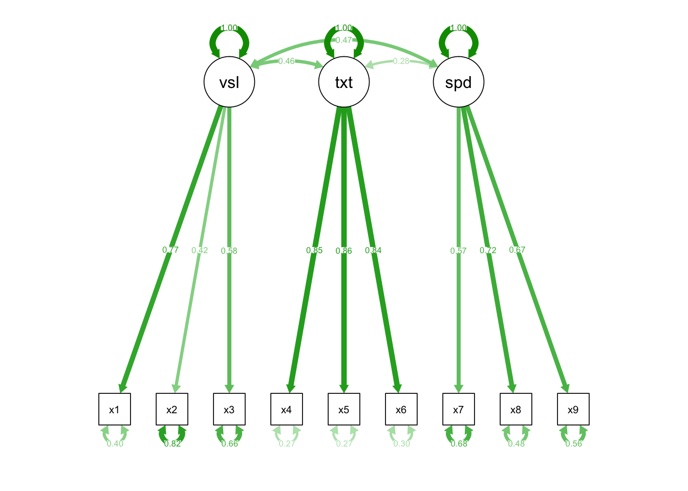
Fixed factor: standardized, unit-free estimates Effects coding: if the original metric is meaningful Marker variable: if you are lazy.
Changes interpretation of some parameters. Will not change fit indices.
7.6.3 Fit Indices
residuals. Good to check.
modification indices. Check to see if missing parameters that residuals may suggest you didn’t include or should include. Can test with more advanced techniques. But eh… makes your models non-theoretical, could be over fitting, relying too much on sig tests…
chi-square. (Statistical fit) Implied versus observed data, tests to see if model are exact fit with data. But eh…too impacted by sample size
RMSEA or SRMR (Absolute fit). Does not compare to a null model. Judges distance from perfect fit.
Above .10 poor fit Below .08 acceptable
- CFI, TFI (Relative fit models). Compares relative to a null model. Judges distance from the worse fit ie a null model. Null models have no covariance among observed and latent variables.
range from 0-1. Indicate % of improvement from the null model to a saturated ie just identified model.
Usually >.9 is okay. Some care about > .95
Minor changes to the model can improve fit.
- Check the model parameters. Are they wonky? Easy to get negative variances or correlations above 1.
7.6.4 Comparing models
Can compare models as in mlm.
anova(model1, model2)Use AIC and BIC, just as with MLM. Smaller values indicate a better fit.
7.6.5 Parcels
It is often necessary to simplify your model. One option to do so is with parcels where you combine indicators into a composite. This simplifies the model in that you have fewer parameters to fit. In addition to being a way to get a model identified, it also has benefits in terms of the assumptions of the indicator variables.
To do so, you can combine items however you want into 3 or 4 groups or parcels, averaging them together. You may balance highly loading with less highly loading items (item to construct technique) or you may pair pos and negatively keyed items together. It is up to you.
Some dislike it because you are aggregating without taking into account the association between the indicators; it is a blind procedure based on theory/assumptions rather than maths. ¯_(ツ)_/¯
7.6.6 Estimators
Default in lavaan is the ML estimator, which we have seen before. There are many other options too, some of which require complete data (though see multiple imputation discussion next class).
There are a number of “robust” estimates that are uniformly better. MLR is my personal choice if you go this route, but others are just as good and maybe better if you have complete data.
To confuse things, there are other methods to get robust standard errors. When data are missing one can request standard errors via a number of different methods. To do so one needs to first specify that data are missing via missing = “ML” in the fitting function. Then use the se function to specify what you want.
Bootstrapped estimates are also available with se = “bootstrap”
7.7 Types of longitudinal models other than growth models (brief intro)
long <- read.csv("~/Box Sync/5165 Applied Longitudinal Data Analysis/SEM_workshop/longitudinal.csv")

summary(long)
## PosAFF11 PosAFF21 PosAFF31 NegAFF11
## Min. :1.365 Min. :0.4152 Min. :1.140 Min. :-0.8584
## 1st Qu.:2.739 1st Qu.:2.6343 1st Qu.:2.797 1st Qu.: 1.1035
## Median :3.209 Median :3.1143 Median :3.204 Median : 1.5075
## Mean :3.212 Mean :3.1050 Mean :3.248 Mean : 1.5220
## 3rd Qu.:3.688 3rd Qu.:3.6216 3rd Qu.:3.775 3rd Qu.: 1.9815
## Max. :5.804 Max. :6.1970 Max. :6.048 Max. : 3.2403
## NegAFF21 NegAFF31 PosAFF12 PosAFF22
## Min. :-0.3991 Min. :-0.5606 Min. :1.528 Min. :0.6575
## 1st Qu.: 1.0229 1st Qu.: 1.0100 1st Qu.:2.852 1st Qu.:2.6571
## Median : 1.3718 Median : 1.4335 Median :3.215 Median :3.1206
## Mean : 1.3971 Mean : 1.3981 Mean :3.253 Mean :3.1256
## 3rd Qu.: 1.7566 3rd Qu.: 1.8101 3rd Qu.:3.637 3rd Qu.:3.5467
## Max. : 2.9844 Max. : 2.7674 Max. :5.413 Max. :5.4420
## PosAFF32 NegAFF12 NegAFF22 NegAFF32
## Min. :0.7369 Min. :0.1797 Min. :0.1784 Min. :-0.03494
## 1st Qu.:2.8484 1st Qu.:1.1464 1st Qu.:0.9963 1st Qu.: 1.02027
## Median :3.2692 Median :1.3818 Median :1.3172 Median : 1.31692
## Mean :3.2737 Mean :1.4115 Mean :1.3237 Mean : 1.30002
## 3rd Qu.:3.7170 3rd Qu.:1.7251 3rd Qu.:1.6382 3rd Qu.: 1.56441
## Max. :5.9676 Max. :2.5033 Max. :2.5587 Max. : 2.44236
## PosAFF13 PosAFF23 PosAFF33 NegAFF13
## Min. :1.307 Min. :0.8057 Min. :1.629 Min. :-0.01837
## 1st Qu.:2.979 1st Qu.:2.7147 1st Qu.:2.858 1st Qu.: 1.15739
## Median :3.299 Median :3.0832 Median :3.325 Median : 1.43937
## Mean :3.302 Mean :3.0945 Mean :3.280 Mean : 1.43015
## 3rd Qu.:3.683 3rd Qu.:3.5296 3rd Qu.:3.698 3rd Qu.: 1.73650
## Max. :4.712 Max. :4.8007 Max. :5.014 Max. : 2.75085
## NegAFF23 NegAFF33
## Min. :0.147 Min. :0.3145
## 1st Qu.:1.009 1st Qu.:1.0261
## Median :1.294 Median :1.3154
## Mean :1.281 Mean :1.2974
## 3rd Qu.:1.560 3rd Qu.:1.5583
## Max. :2.447 Max. :2.63857.7.1 Longitudinal CFA
key concerns: 1. Should the correlations be the same across time? 2. Should the error variances be correlated? 3. Are the loadings the same across time? (more on this later)
long.cfa <- '
## define latent variables
Pos1 =~ PosAFF11 + PosAFF21 + PosAFF31
Pos2 =~ PosAFF12 + PosAFF22 + PosAFF32
Pos3 =~ PosAFF13 + PosAFF23 + PosAFF33
Neg1 =~ NegAFF11 + NegAFF21 + NegAFF31
Neg2 =~ NegAFF12 + NegAFF22 + NegAFF32
Neg3 =~ NegAFF13 + NegAFF23 + NegAFF33

## correlated residuals across time
PosAFF11 ~~ PosAFF12 + PosAFF13
PosAFF12 ~~ PosAFF13
PosAFF21 ~~ PosAFF22 + PosAFF23
PosAFF22 ~~ PosAFF23
PosAFF31 ~~ PosAFF32 + PosAFF33
PosAFF32 ~~ PosAFF33

NegAFF11 ~~ NegAFF12 + NegAFF13
NegAFF12 ~~ NegAFF13
NegAFF21 ~~ NegAFF22 + NegAFF23
NegAFF22 ~~ NegAFF23
NegAFF31 ~~ NegAFF32 + NegAFF33
NegAFF32 ~~ NegAFF33

'

fit.long.cfa <- cfa(long.cfa, data=long, std.lv=TRUE)

summary(fit.long.cfa, standardized=TRUE, fit.measures=TRUE)
## lavaan (0.5-23.1097) converged normally after 134 iterations
##
## Number of observations 368
##
## Estimator ML
## Minimum Function Test Statistic 119.443
## Degrees of freedom 102
## P-value (Chi-square) 0.114
##
## Model test baseline model:
##
## Minimum Function Test Statistic 5253.085
## Degrees of freedom 153
## P-value 0.000
##
## User model versus baseline model:
##
## Comparative Fit Index (CFI) 0.997
## Tucker-Lewis Index (TLI) 0.995
##
## Loglikelihood and Information Criteria:
##
## Loglikelihood user model (H0) -3060.353
## Loglikelihood unrestricted model (H1) -3000.632
##
## Number of free parameters 69
## Akaike (AIC) 6258.707
## Bayesian (BIC) 6528.365
## Sample-size adjusted Bayesian (BIC) 6309.453
##
## Root Mean Square Error of Approximation:
##
## RMSEA 0.022
## 90 Percent Confidence Interval 0.000 0.036
## P-value RMSEA <= 0.05 1.000
##
## Standardized Root Mean Square Residual:
##
## SRMR 0.028
##
## Parameter Estimates:
##
## Information Expected
## Standard Errors Standard
##
## Latent Variables:
## Estimate Std.Err z-value P(>|z|) Std.lv Std.all
## Pos1 =~
## PosAFF11 0.654 0.030 21.936 0.000 0.654 0.903
## PosAFF21 0.651 0.031 20.864 0.000 0.651 0.875
## PosAFF31 0.685 0.031 22.361 0.000 0.685 0.912
## Pos2 =~
## PosAFF12 0.556 0.026 21.256 0.000 0.556 0.883
## PosAFF22 0.638 0.030 21.448 0.000 0.638 0.887
## PosAFF32 0.644 0.027 23.567 0.000 0.644 0.940
## Pos3 =~
## PosAFF13 0.508 0.024 21.028 0.000 0.508 0.887
## PosAFF23 0.545 0.027 20.347 0.000 0.545 0.867
## PosAFF33 0.538 0.026 20.827 0.000 0.538 0.879
## Neg1 =~
## NegAFF11 0.563 0.028 20.465 0.000 0.563 0.868
## NegAFF21 0.479 0.024 19.856 0.000 0.479 0.847
## NegAFF31 0.555 0.025 22.373 0.000 0.555 0.920
## Neg2 =~
## NegAFF12 0.365 0.019 18.989 0.000 0.365 0.826
## NegAFF22 0.375 0.017 21.452 0.000 0.375 0.889
## NegAFF32 0.368 0.017 21.383 0.000 0.368 0.896
## Neg3 =~
## NegAFF13 0.363 0.021 17.128 0.000 0.363 0.782
## NegAFF23 0.341 0.017 19.493 0.000 0.341 0.855
## NegAFF33 0.344 0.017 19.700 0.000 0.344 0.869
##
## Covariances:
## Estimate Std.Err z-value P(>|z|) Std.lv Std.all
## .PosAFF11 ~~
## .PosAFF12 0.004 0.007 0.578 0.563 0.004 0.043
## .PosAFF13 0.000 0.007 0.037 0.971 0.000 0.003
## .PosAFF12 ~~
## .PosAFF13 0.004 0.006 0.674 0.500 0.004 0.050
## .PosAFF21 ~~
## .PosAFF22 0.008 0.008 1.020 0.308 0.008 0.071
## .PosAFF23 0.008 0.008 0.991 0.322 0.008 0.070
## .PosAFF22 ~~
## .PosAFF23 0.011 0.007 1.470 0.142 0.011 0.104
## .PosAFF31 ~~
## .PosAFF32 0.004 0.007 0.616 0.538 0.004 0.057
## .PosAFF33 0.016 0.007 2.182 0.029 0.016 0.177
## .PosAFF32 ~~
## .PosAFF33 0.004 0.006 0.690 0.490 0.004 0.061
## .NegAFF11 ~~
## .NegAFF12 0.005 0.005 0.966 0.334 0.005 0.065
## .NegAFF13 0.006 0.006 1.036 0.300 0.006 0.070
## .NegAFF12 ~~
## .NegAFF13 0.007 0.005 1.528 0.126 0.007 0.099
## .NegAFF21 ~~
## .NegAFF22 0.015 0.004 3.605 0.000 0.015 0.267
## .NegAFF23 0.011 0.005 2.387 0.017 0.011 0.173
## .NegAFF22 ~~
## .NegAFF23 0.010 0.003 3.145 0.002 0.010 0.253
## .NegAFF31 ~~
## .NegAFF32 -0.006 0.004 -1.607 0.108 -0.006 -0.147
## .NegAFF33 -0.008 0.004 -1.778 0.075 -0.008 -0.163
## .NegAFF32 ~~
## .NegAFF33 -0.001 0.003 -0.481 0.630 -0.001 -0.041
## Pos1 ~~
## Pos2 0.473 0.044 10.663 0.000 0.473 0.473
## Pos3 0.399 0.048 8.228 0.000 0.399 0.399
## Neg1 -0.436 0.047 -9.358 0.000 -0.436 -0.436
## Neg2 -0.297 0.052 -5.706 0.000 -0.297 -0.297
## Neg3 -0.169 0.056 -3.003 0.003 -0.169 -0.169
## Pos2 ~~
## Pos3 0.449 0.046 9.777 0.000 0.449 0.449
## Neg1 -0.179 0.054 -3.279 0.001 -0.179 -0.179
## Neg2 -0.543 0.041 -13.203 0.000 -0.543 -0.543
## Neg3 -0.198 0.055 -3.578 0.000 -0.198 -0.198
## Pos3 ~~
## Neg1 -0.074 0.057 -1.304 0.192 -0.074 -0.074
## Neg2 -0.167 0.056 -2.989 0.003 -0.167 -0.167
## Neg3 -0.292 0.054 -5.442 0.000 -0.292 -0.292
## Neg1 ~~
## Neg2 0.526 0.043 12.317 0.000 0.526 0.526
## Neg3 0.351 0.052 6.778 0.000 0.351 0.351
## Neg2 ~~
## Neg3 0.435 0.048 9.006 0.000 0.435 0.435
##
## Variances:
## Estimate Std.Err z-value P(>|z|) Std.lv Std.all
## .PosAFF11 0.096 0.011 8.497 0.000 0.096 0.184
## .PosAFF21 0.130 0.013 9.956 0.000 0.130 0.235
## .PosAFF31 0.095 0.012 7.944 0.000 0.095 0.168
## .PosAFF12 0.087 0.009 10.044 0.000 0.087 0.220
## .PosAFF22 0.110 0.011 9.883 0.000 0.110 0.213
## .PosAFF32 0.055 0.009 6.437 0.000 0.055 0.117
## .PosAFF13 0.070 0.008 8.319 0.000 0.070 0.214
## .PosAFF23 0.098 0.011 9.317 0.000 0.098 0.249
## .PosAFF33 0.085 0.010 8.716 0.000 0.085 0.227
## .NegAFF11 0.104 0.011 9.546 0.000 0.104 0.246
## .NegAFF21 0.091 0.009 10.363 0.000 0.091 0.283
## .NegAFF31 0.056 0.009 6.475 0.000 0.056 0.153
## .NegAFF12 0.062 0.006 10.835 0.000 0.062 0.317
## .NegAFF22 0.037 0.004 8.445 0.000 0.037 0.209
## .NegAFF32 0.033 0.004 7.917 0.000 0.033 0.198
## .NegAFF13 0.084 0.008 10.660 0.000 0.084 0.389
## .NegAFF23 0.043 0.005 8.170 0.000 0.043 0.270
## .NegAFF33 0.038 0.005 7.372 0.000 0.038 0.245
## Pos1 1.000 1.000 1.000
## Pos2 1.000 1.000 1.000
## Pos3 1.000 1.000 1.000
## Neg1 1.000 1.000 1.000
## Neg2 1.000 1.000 1.000
## Neg3 1.000 1.000 1.000semPaths(fit.long.cfa)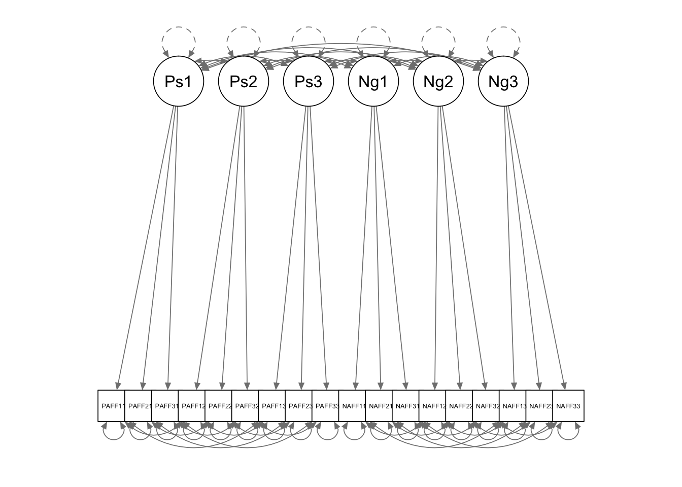
7.7.2 Longitudinal Path Model
key concerns: 1. Should the regressions be the same across time? 2. Should the error variances be correlated? 3. Are the loadings the same across time? (more on this later)
long.path <- '
## define latent variables
Pos1 =~ L1*PosAFF11 + L2*PosAFF21 + L3*PosAFF31
Pos2 =~ L1*PosAFF12 + L2*PosAFF22 + L3*PosAFF32
Pos3 =~ L1*PosAFF13 + L2*PosAFF23 + L3*PosAFF33
Neg1 =~ L4*NegAFF11 + L5*NegAFF21 + L6*NegAFF31
Neg2 =~ L4*NegAFF12 + L5*NegAFF22 + L6*NegAFF32
Neg3 =~ L4*NegAFF13 + L5*NegAFF23 + L6*NegAFF33

## free latent variances at later times (only set the scale once)
Pos2 ~~ NA*Pos2
Pos3 ~~ NA*Pos3
Neg2 ~~ NA*Neg2
Neg3 ~~ NA*Neg3
Pos1 ~~ Neg1
Pos2 ~~ Neg2
Pos3 ~~ Neg3

## directional regression paths
Pos2 ~ Pos1
Pos3 ~ Pos2
Neg2 ~ Neg1
Neg3 ~ Neg2

## correlated residuals across time
PosAFF11 ~~ PosAFF12 + PosAFF13
PosAFF12 ~~ PosAFF13
PosAFF21 ~~ PosAFF22 + PosAFF23
PosAFF22 ~~ PosAFF23
PosAFF31 ~~ PosAFF32 + PosAFF33
PosAFF32 ~~ PosAFF33

NegAFF11 ~~ NegAFF12 + NegAFF13
NegAFF12 ~~ NegAFF13
NegAFF21 ~~ NegAFF22 + NegAFF23
NegAFF22 ~~ NegAFF23
NegAFF31 ~~ NegAFF32 + NegAFF33
NegAFF32 ~~ NegAFF33
'

fit.long.path <- sem(long.path, data=long, std.lv=TRUE)

summary(fit.long.path, standardized=TRUE, fit.measures=TRUE)
## lavaan (0.5-23.1097) converged normally after 141 iterations
##
## Number of observations 368
##
## Estimator ML
## Minimum Function Test Statistic 170.843
## Degrees of freedom 118
## P-value (Chi-square) 0.001
##
## Model test baseline model:
##
## Minimum Function Test Statistic 5253.085
## Degrees of freedom 153
## P-value 0.000
##
## User model versus baseline model:
##
## Comparative Fit Index (CFI) 0.990
## Tucker-Lewis Index (TLI) 0.987
##
## Loglikelihood and Information Criteria:
##
## Loglikelihood user model (H0) -3086.053
## Loglikelihood unrestricted model (H1) -3000.632
##
## Number of free parameters 53
## Akaike (AIC) 6278.107
## Bayesian (BIC) 6485.235
## Sample-size adjusted Bayesian (BIC) 6317.086
##
## Root Mean Square Error of Approximation:
##
## RMSEA 0.035
## 90 Percent Confidence Interval 0.023 0.046
## P-value RMSEA <= 0.05 0.989
##
## Standardized Root Mean Square Residual:
##
## SRMR 0.055
##
## Parameter Estimates:
##
## Information Expected
## Standard Errors Standard
##
## Latent Variables:
## Estimate Std.Err z-value P(>|z|) Std.lv Std.all
## Pos1 =~
## PosAFF11 (L1) 0.630 0.027 23.609 0.000 0.630 0.892
## PosAFF21 (L2) 0.673 0.029 23.387 0.000 0.673 0.884
## PosAFF31 (L3) 0.686 0.029 23.966 0.000 0.686 0.913
## Pos2 =~
## PosAFF12 (L1) 0.630 0.027 23.609 0.000 0.575 0.893
## PosAFF22 (L2) 0.673 0.029 23.387 0.000 0.614 0.878
## PosAFF32 (L3) 0.686 0.029 23.966 0.000 0.626 0.932
## Pos3 =~
## PosAFF13 (L1) 0.630 0.027 23.609 0.000 0.504 0.884
## PosAFF23 (L2) 0.673 0.029 23.387 0.000 0.539 0.861
## PosAFF33 (L3) 0.686 0.029 23.966 0.000 0.549 0.887
## Neg1 =~
## NegAFF11 (L4) 0.546 0.024 22.398 0.000 0.546 0.859
## NegAFF21 (L5) 0.510 0.023 22.505 0.000 0.510 0.868
## NegAFF31 (L6) 0.537 0.023 23.717 0.000 0.537 0.908
## Neg2 =~
## NegAFF12 (L4) 0.546 0.024 22.398 0.000 0.384 0.841
## NegAFF22 (L5) 0.510 0.023 22.505 0.000 0.358 0.871
## NegAFF32 (L6) 0.537 0.023 23.717 0.000 0.377 0.904
## Neg3 =~
## NegAFF13 (L4) 0.546 0.024 22.398 0.000 0.362 0.780
## NegAFF23 (L5) 0.510 0.023 22.505 0.000 0.338 0.847
## NegAFF33 (L6) 0.537 0.023 23.717 0.000 0.356 0.883
##
## Regressions:
## Estimate Std.Err z-value P(>|z|) Std.lv Std.all
## Pos2 ~
## Pos1 0.416 0.042 10.020 0.000 0.456 0.456
## Pos3 ~
## Pos2 0.404 0.044 9.207 0.000 0.460 0.460
## Neg2 ~
## Neg1 0.382 0.031 12.203 0.000 0.544 0.544
## Neg3 ~
## Neg2 0.432 0.049 8.867 0.000 0.457 0.457
##
## Covariances:
## Estimate Std.Err z-value P(>|z|) Std.lv Std.all
## Pos1 ~~
## Neg1 -0.441 0.046 -9.502 0.000 -0.441 -0.441
## .Pos2 ~~
## .Neg2 -0.269 0.036 -7.544 0.000 -0.561 -0.561
## .Pos3 ~~
## .Neg3 -0.125 0.027 -4.596 0.000 -0.298 -0.298
## .PosAFF11 ~~
## .PosAFF12 0.004 0.007 0.536 0.592 0.004 0.039
## .PosAFF13 0.003 0.007 0.386 0.699 0.003 0.030
## .PosAFF12 ~~
## .PosAFF13 0.003 0.006 0.585 0.559 0.003 0.044
## .PosAFF21 ~~
## .PosAFF22 0.007 0.008 0.865 0.387 0.007 0.061
## .PosAFF23 0.008 0.008 1.030 0.303 0.008 0.074
## .PosAFF22 ~~
## .PosAFF23 0.011 0.007 1.516 0.130 0.011 0.106
## .PosAFF31 ~~
## .PosAFF32 0.005 0.007 0.705 0.481 0.005 0.064
## .PosAFF33 0.016 0.007 2.173 0.030 0.016 0.180
## .PosAFF32 ~~
## .PosAFF33 0.004 0.006 0.580 0.562 0.004 0.051
## .NegAFF11 ~~
## .NegAFF12 0.005 0.005 0.947 0.344 0.005 0.064
## .NegAFF13 0.007 0.006 1.107 0.268 0.007 0.073
## .NegAFF12 ~~
## .NegAFF13 0.007 0.005 1.539 0.124 0.007 0.100
## .NegAFF21 ~~
## .NegAFF22 0.015 0.004 3.399 0.001 0.015 0.249
## .NegAFF23 0.010 0.005 2.217 0.027 0.010 0.163
## .NegAFF22 ~~
## .NegAFF23 0.011 0.003 3.430 0.001 0.011 0.259
## .NegAFF31 ~~
## .NegAFF32 -0.007 0.004 -1.724 0.085 -0.007 -0.155
## .NegAFF33 -0.007 0.004 -1.587 0.113 -0.007 -0.143
## .NegAFF32 ~~
## .NegAFF33 -0.002 0.003 -0.734 0.463 -0.002 -0.066
##
## Variances:
## Estimate Std.Err z-value P(>|z|) Std.lv Std.all
## .Pos2 0.660 0.075 8.760 0.000 0.792 0.792
## .Pos3 0.504 0.058 8.628 0.000 0.788 0.788
## .Neg2 0.347 0.041 8.458 0.000 0.704 0.704
## .Neg3 0.347 0.041 8.409 0.000 0.791 0.791
## .PosAFF11 0.102 0.011 9.329 0.000 0.102 0.204
## .PosAFF21 0.126 0.013 9.699 0.000 0.126 0.218
## .PosAFF31 0.094 0.012 8.132 0.000 0.094 0.166
## .PosAFF12 0.084 0.009 9.650 0.000 0.084 0.202
## .PosAFF22 0.112 0.011 10.307 0.000 0.112 0.229
## .PosAFF32 0.059 0.008 7.215 0.000 0.059 0.131
## .PosAFF13 0.071 0.008 8.813 0.000 0.071 0.218
## .PosAFF23 0.101 0.010 9.833 0.000 0.101 0.259
## .PosAFF33 0.082 0.009 8.703 0.000 0.082 0.214
## .NegAFF11 0.106 0.010 10.098 0.000 0.106 0.262
## .NegAFF21 0.085 0.009 9.768 0.000 0.085 0.247
## .NegAFF31 0.062 0.008 7.633 0.000 0.062 0.176
## .NegAFF12 0.061 0.006 10.625 0.000 0.061 0.292
## .NegAFF22 0.041 0.004 9.619 0.000 0.041 0.242
## .NegAFF32 0.032 0.004 7.781 0.000 0.032 0.182
## .NegAFF13 0.084 0.008 11.031 0.000 0.084 0.392
## .NegAFF23 0.045 0.005 9.102 0.000 0.045 0.282
## .NegAFF33 0.036 0.005 7.466 0.000 0.036 0.221
## Pos1 1.000 1.000 1.000
## Neg1 1.000 1.000 1.000semPaths(fit.long.path, layout = "tree3")
## layout can also be done manually to get publications worthy plots7.7.3 Longitudinal Cross lagged model
key concerns: 1. Should the regressions (both cross lagged and autoregressive) be the same across time? 2. Should the indicator error variances be correlated (within time or within construct)? 3. Are the loadings the same across time? (more on this later) 4. Are the latent error variances the same or different? 5. Are the latent error variances correlated the same or different across time? 6. Are there more lagged effects?
long.cross <- '
## define latent variables
Pos1 =~ L1*PosAFF11 + L2*PosAFF21 + L3*PosAFF31
Pos2 =~ L1*PosAFF12 + L2*PosAFF22 + L3*PosAFF32
Pos3 =~ L1*PosAFF13 + L2*PosAFF23 + L3*PosAFF33
Neg1 =~ L4*NegAFF11 + L5*NegAFF21 + L6*NegAFF31
Neg2 =~ L4*NegAFF12 + L5*NegAFF22 + L6*NegAFF32
Neg3 =~ L4*NegAFF13 + L5*NegAFF23 + L6*NegAFF33

## free latent variances at later times (only set the scale once)
Pos2 ~~ NA*Pos2
Pos3 ~~ NA*Pos3
Neg2 ~~ NA*Neg2
Neg3 ~~ NA*Neg3

Pos1 ~~ Neg1
Pos2 ~~ Neg2
Pos3 ~~ Neg3

## directional regression paths
Pos2 ~ Pos1 + Neg1
Neg2 ~ Pos1 + Neg1
Pos3 ~ Pos2 + Neg2
Neg3 ~ Pos2 + Neg2

## correlated residuals across time
PosAFF11 ~~ PosAFF12 + PosAFF13
PosAFF12 ~~ PosAFF13
PosAFF21 ~~ PosAFF22 + PosAFF23
PosAFF22 ~~ PosAFF23
PosAFF31 ~~ PosAFF32 + PosAFF33
PosAFF32 ~~ PosAFF33

NegAFF11 ~~ NegAFF12 + NegAFF13
NegAFF12 ~~ NegAFF13
NegAFF21 ~~ NegAFF22 + NegAFF23
NegAFF22 ~~ NegAFF23
NegAFF31 ~~ NegAFF32 + NegAFF33
NegAFF32 ~~ NegAFF33
'

fit.long.cross <- sem(long.cross,data=long, std.lv=TRUE)

summary(fit.long.cross, standardized=TRUE, fit.measures=TRUE)
## lavaan (0.5-23.1097) converged normally after 151 iterations
##
## Number of observations 368
##
## Estimator ML
## Minimum Function Test Statistic 163.406
## Degrees of freedom 114
## P-value (Chi-square) 0.002
##
## Model test baseline model:
##
## Minimum Function Test Statistic 5253.085
## Degrees of freedom 153
## P-value 0.000
##
## User model versus baseline model:
##
## Comparative Fit Index (CFI) 0.990
## Tucker-Lewis Index (TLI) 0.987
##
## Loglikelihood and Information Criteria:
##
## Loglikelihood user model (H0) -3082.335
## Loglikelihood unrestricted model (H1) -3000.632
##
## Number of free parameters 57
## Akaike (AIC) 6278.669
## Bayesian (BIC) 6501.430
## Sample-size adjusted Bayesian (BIC) 6320.590
##
## Root Mean Square Error of Approximation:
##
## RMSEA 0.034
## 90 Percent Confidence Interval 0.022 0.046
## P-value RMSEA <= 0.05 0.990
##
## Standardized Root Mean Square Residual:
##
## SRMR 0.051
##
## Parameter Estimates:
##
## Information Expected
## Standard Errors Standard
##
## Latent Variables:
## Estimate Std.Err z-value P(>|z|) Std.lv Std.all
## Pos1 =~
## PosAFF11 (L1) 0.630 0.027 23.619 0.000 0.630 0.892
## PosAFF21 (L2) 0.673 0.029 23.393 0.000 0.673 0.884
## PosAFF31 (L3) 0.686 0.029 23.990 0.000 0.686 0.914
## Pos2 =~
## PosAFF12 (L1) 0.630 0.027 23.619 0.000 0.582 0.896
## PosAFF22 (L2) 0.673 0.029 23.393 0.000 0.622 0.880
## PosAFF32 (L3) 0.686 0.029 23.990 0.000 0.634 0.933
## Pos3 =~
## PosAFF13 (L1) 0.630 0.027 23.619 0.000 0.503 0.884
## PosAFF23 (L2) 0.673 0.029 23.393 0.000 0.537 0.861
## PosAFF33 (L3) 0.686 0.029 23.990 0.000 0.547 0.886
## Neg1 =~
## NegAFF11 (L4) 0.547 0.024 22.394 0.000 0.547 0.860
## NegAFF21 (L5) 0.510 0.023 22.488 0.000 0.510 0.868
## NegAFF31 (L6) 0.538 0.023 23.710 0.000 0.538 0.908
## Neg2 =~
## NegAFF12 (L4) 0.547 0.024 22.394 0.000 0.382 0.840
## NegAFF22 (L5) 0.510 0.023 22.488 0.000 0.356 0.869
## NegAFF32 (L6) 0.538 0.023 23.710 0.000 0.375 0.903
## Neg3 =~
## NegAFF13 (L4) 0.547 0.024 22.394 0.000 0.358 0.777
## NegAFF23 (L5) 0.510 0.023 22.488 0.000 0.334 0.844
## NegAFF33 (L6) 0.538 0.023 23.710 0.000 0.352 0.881
##
## Regressions:
## Estimate Std.Err z-value P(>|z|) Std.lv Std.all
## Pos2 ~
## Pos1 0.463 0.052 8.829 0.000 0.501 0.501
## Neg1 0.039 0.053 0.746 0.456 0.042 0.042
## Neg2 ~
## Pos1 -0.057 0.039 -1.454 0.146 -0.081 -0.081
## Neg1 0.347 0.039 8.812 0.000 0.498 0.498
## Pos3 ~
## Pos2 0.451 0.054 8.307 0.000 0.522 0.522
## Neg2 0.134 0.073 1.843 0.065 0.117 0.117
## Neg3 ~
## Pos2 0.046 0.046 1.000 0.317 0.065 0.065
## Neg2 0.446 0.062 7.239 0.000 0.475 0.475
##
## Covariances:
## Estimate Std.Err z-value P(>|z|) Std.lv Std.all
## Pos1 ~~
## Neg1 -0.437 0.047 -9.375 0.000 -0.437 -0.437
## .Pos2 ~~
## .Neg2 -0.269 0.036 -7.567 0.000 -0.566 -0.566
## .Pos3 ~~
## .Neg3 -0.127 0.027 -4.711 0.000 -0.308 -0.308
## .PosAFF11 ~~
## .PosAFF12 0.004 0.007 0.529 0.597 0.004 0.039
## .PosAFF13 0.002 0.007 0.371 0.711 0.002 0.028
## .PosAFF12 ~~
## .PosAFF13 0.003 0.006 0.569 0.569 0.003 0.043
## .PosAFF21 ~~
## .PosAFF22 0.007 0.008 0.869 0.385 0.007 0.061
## .PosAFF23 0.008 0.008 0.964 0.335 0.008 0.069
## .PosAFF22 ~~
## .PosAFF23 0.011 0.007 1.416 0.157 0.011 0.099
## .PosAFF31 ~~
## .PosAFF32 0.004 0.007 0.649 0.516 0.004 0.059
## .PosAFF33 0.016 0.007 2.257 0.024 0.016 0.187
## .PosAFF32 ~~
## .PosAFF33 0.004 0.006 0.580 0.562 0.004 0.050
## .NegAFF11 ~~
## .NegAFF12 0.005 0.005 0.986 0.324 0.005 0.067
## .NegAFF13 0.007 0.006 1.088 0.277 0.007 0.072
## .NegAFF12 ~~
## .NegAFF13 0.007 0.005 1.537 0.124 0.007 0.100
## .NegAFF21 ~~
## .NegAFF22 0.015 0.004 3.440 0.001 0.015 0.252
## .NegAFF23 0.010 0.005 2.238 0.025 0.010 0.165
## .NegAFF22 ~~
## .NegAFF23 0.011 0.003 3.397 0.001 0.011 0.256
## .NegAFF31 ~~
## .NegAFF32 -0.007 0.004 -1.748 0.080 -0.007 -0.157
## .NegAFF33 -0.007 0.004 -1.602 0.109 -0.007 -0.145
## .NegAFF32 ~~
## .NegAFF33 -0.002 0.003 -0.751 0.453 -0.002 -0.068
##
## Variances:
## Estimate Std.Err z-value P(>|z|) Std.lv Std.all
## .Pos2 0.653 0.075 8.735 0.000 0.765 0.765
## .Pos3 0.496 0.058 8.594 0.000 0.780 0.780
## .Neg2 0.346 0.041 8.475 0.000 0.710 0.710
## .Neg3 0.345 0.041 8.396 0.000 0.804 0.804
## .PosAFF11 0.102 0.011 9.359 0.000 0.102 0.205
## .PosAFF21 0.127 0.013 9.731 0.000 0.127 0.219
## .PosAFF31 0.093 0.012 8.100 0.000 0.093 0.165
## .PosAFF12 0.083 0.009 9.656 0.000 0.083 0.198
## .PosAFF22 0.113 0.011 10.344 0.000 0.113 0.226
## .PosAFF32 0.060 0.008 7.270 0.000 0.060 0.129
## .PosAFF13 0.071 0.008 8.814 0.000 0.071 0.219
## .PosAFF23 0.101 0.010 9.817 0.000 0.101 0.259
## .PosAFF33 0.082 0.009 8.730 0.000 0.082 0.216
## .NegAFF11 0.105 0.010 10.063 0.000 0.105 0.260
## .NegAFF21 0.085 0.009 9.775 0.000 0.085 0.247
## .NegAFF31 0.062 0.008 7.599 0.000 0.062 0.176
## .NegAFF12 0.061 0.006 10.647 0.000 0.061 0.295
## .NegAFF22 0.041 0.004 9.668 0.000 0.041 0.245
## .NegAFF32 0.032 0.004 7.810 0.000 0.032 0.184
## .NegAFF13 0.084 0.008 11.023 0.000 0.084 0.396
## .NegAFF23 0.045 0.005 9.106 0.000 0.045 0.287
## .NegAFF33 0.036 0.005 7.452 0.000 0.036 0.224
## Pos1 1.000 1.000 1.000
## Neg1 1.000 1.000 1.000semPaths(fit.long.cross)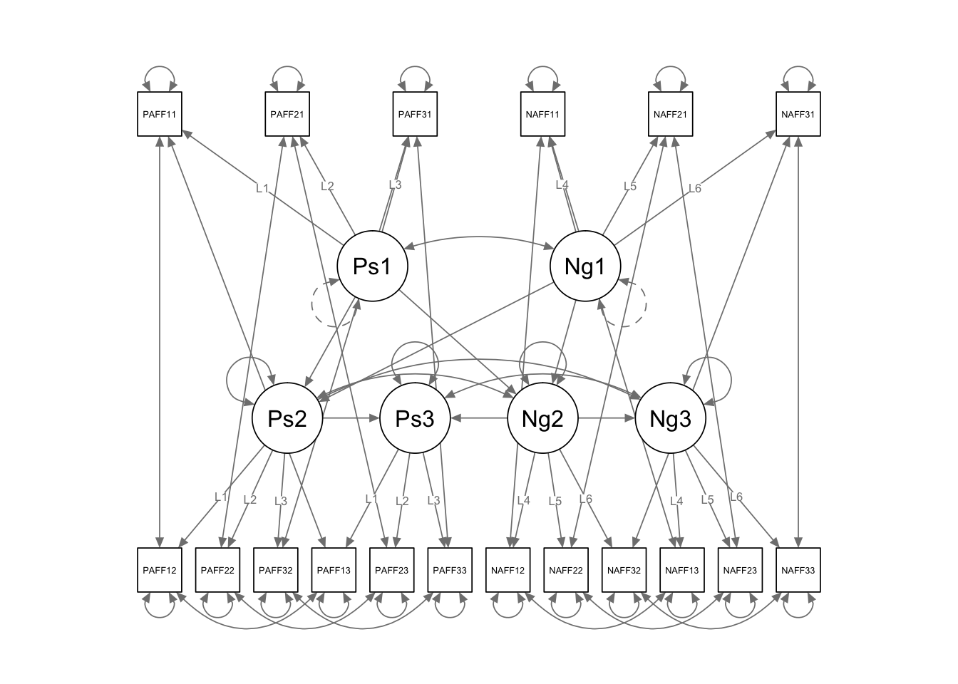
semPaths(fit.long.cross, layout = "tree3")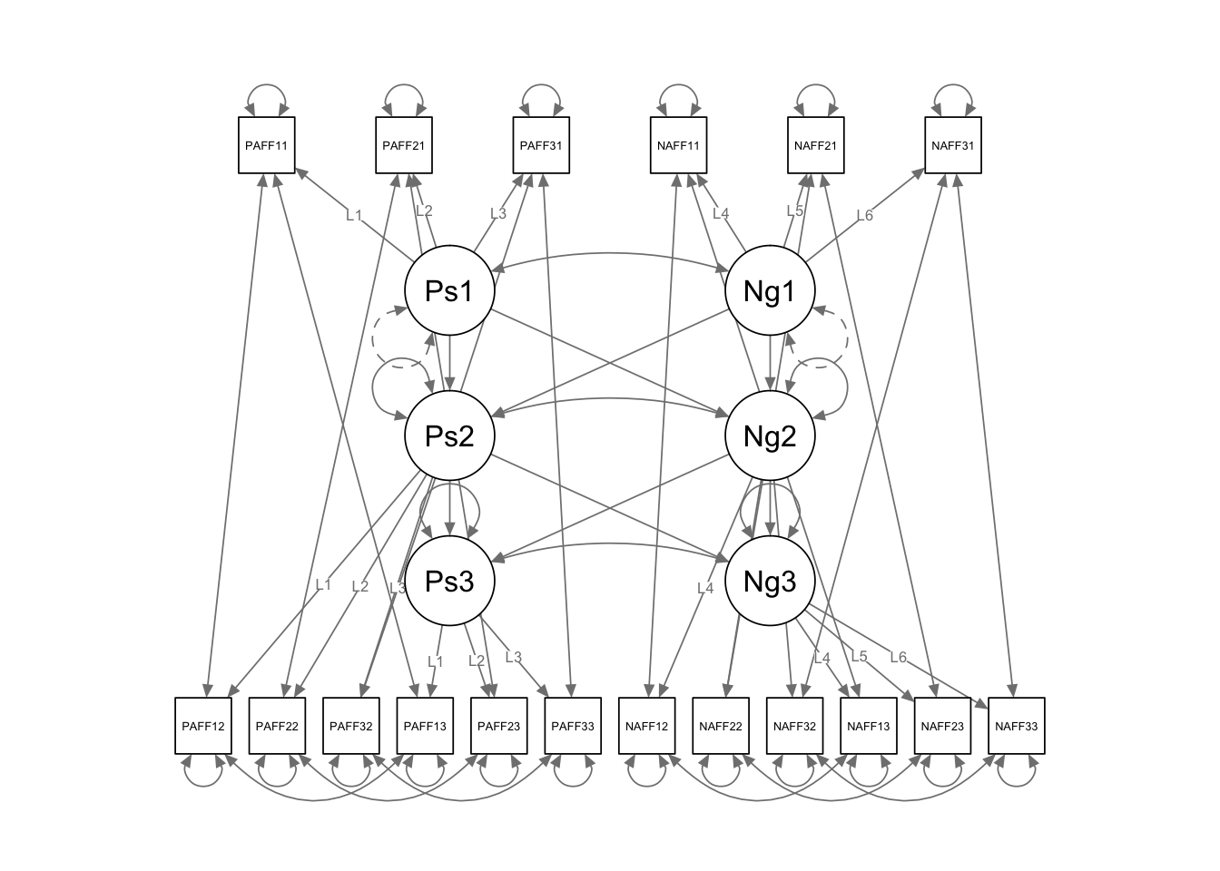
7.7.4 Longitudinal mediation model
#Do Self-Reported Social Experiences Mediate the Effect of Extraversion on Life Satisfaction and Happiness?
#number close friends
library(readr)
TSS_sub <- read_csv("~/Box Sync/5165 Applied Longitudinal Data Analysis/Longitudinal/TSS_sub.csv")
## Warning: Missing column names filled in: 'X1' [1]## Parsed with column specification:
## cols(
## .default = col_integer(),
## a1bfie = col_double(),
## a1bfia = col_double(),
## a1bfic = col_double(),
## a1bfin = col_double(),
## a1bfio = col_double(),
## a1panpos = col_double(),
## a1panneg = col_double(),
## f1gpa = col_double(),
## f1sbcad = col_double(),
## f1gpaes = col_double(),
## f1acwkp = col_double(),
## f1acvol = col_double(),
## f1acode = col_character(),
## f1acohr = col_double(),
## f1mhpro = col_double(),
## h1gpaes = col_double(),
## h1gpafr = col_double(),
## h1acwkp = col_double(),
## h1acvol = col_double(),
## h1acspo = col_double()
## # ... with 114 more columns
## )## See spec(...) for full column specifications.scon.model6<-'
# definine extraversion
bfie =~ a1bfi01 + a1bfi06r + a1bfi11 + a1bfi16 + a1bfi21r + a1bfi26 + a1bfi31r + a1bfi36
# correlated residuals
a1bfi11 ~~ a1bfi16
a1bfi06r ~~ a1bfi21r + a1bfi31r
a1bfi21r ~~ a1bfi31r + a1bfi01
#define social connection at 4 waves
hconnect=~h1clrel + h1satfr + h1sosat + h1ced05
jconnect=~j1clrel + j1satfr + j1sosat + j1ced05
kconnect=~k1clrel + k1satfr + k1sosat + k1ced05
mconnect=~m1clrel + m1satfr + m1sosat + m1ced05
#correlate residuals
h1clrel ~~ j1clrel + k1clrel + m1clrel
j1clrel ~~ k1clrel + m1clrel
k1clrel ~~ m1clrel
h1satfr ~~ j1satfr + k1satfr + m1satfr
j1satfr ~~ k1satfr + m1satfr
k1satfr ~~ m1satfr
h1sosat ~~ j1sosat + k1sosat + m1sosat
j1sosat ~~ k1sosat + m1sosat
k1sosat ~~ m1sosat
h1ced05 ~~ j1ced05 + k1ced05 + m1ced05
j1ced05 ~~ k1ced05 + m1ced05
k1ced05 ~~ m1ced05
# same time covariances between extraversion, connection, satisfaction
bfie~~a1swls
hconnect ~~ h1swls
jconnect ~~ j1swls
kconnect ~~ k1swls
#regressions to calculate indiret effects
hconnect ~ a1*bfie + d1*a1swls
jconnect ~ a2*bfie + d2*h1swls + m1*hconnect
kconnect ~ a3*bfie + d3*j1swls + m2*jconnect
mconnect ~ a4*bfie + d4*k1swls + m3*kconnect
h1swls ~ y1*a1swls + c1*bfie
j1swls ~ y2*h1swls + c2*bfie + b1*hconnect
k1swls ~ y3*j1swls + c3*bfie + b2*jconnect
m1swls ~ y4*k1swls + c4*bfie + b3*kconnect
#effects
# extraversion -> connect (a)
# connect -> swb (b)
# extraversion -> swb (c)
# auto-regressive connection (m)
# auto-regressive swb (y)
ind:= a1*b1*y3*y4 + a1*m1*b2*y4 + a1*m1*m2*b3 + a2*b2*y4 + a2*m2*b3 + a3*b3
total:= ind + c4 + c3*y4 + c2*y3*y4 + c1*y2*y3*y4
'
scon62 <- sem(scon.model6, data=TSS_sub, missing = "ml", fixed.x = FALSE)
summary(scon62, standardized=T, fit.measures=TRUE)## lavaan (0.5-23.1097) converged normally after 113 iterations
##
## Number of observations 393
##
## Number of missing patterns 30
##
## Estimator ML
## Minimum Function Test Statistic 600.051
## Degrees of freedom 326
## P-value (Chi-square) 0.000
##
## Model test baseline model:
##
## Minimum Function Test Statistic 4447.119
## Degrees of freedom 406
## P-value 0.000
##
## User model versus baseline model:
##
## Comparative Fit Index (CFI) 0.932
## Tucker-Lewis Index (TLI) 0.916
##
## Loglikelihood and Information Criteria:
##
## Loglikelihood user model (H0) -13558.593
## Loglikelihood unrestricted model (H1) -13258.568
##
## Number of free parameters 138
## Akaike (AIC) 27393.187
## Bayesian (BIC) 27941.573
## Sample-size adjusted Bayesian (BIC) 27503.702
##
## Root Mean Square Error of Approximation:
##
## RMSEA 0.046
## 90 Percent Confidence Interval 0.040 0.052
## P-value RMSEA <= 0.05 0.854
##
## Standardized Root Mean Square Residual:
##
## SRMR 0.068
##
## Parameter Estimates:
##
## Information Observed
## Standard Errors Standard
##
## Latent Variables:
## Estimate Std.Err z-value P(>|z|) Std.lv Std.all
## bfie =~
## a1bfi01 1.000 0.905 0.728
## a1bfi06r 0.813 0.072 11.336 0.000 0.735 0.601
## a1bfi11 0.605 0.056 10.808 0.000 0.547 0.592
## a1bfi16 0.603 0.054 11.084 0.000 0.545 0.604
## a1bfi21r 0.951 0.063 15.013 0.000 0.860 0.700
## a1bfi26 0.806 0.067 12.066 0.000 0.729 0.648
## a1bfi31r 0.823 0.072 11.471 0.000 0.744 0.618
## a1bfi36 1.064 0.068 15.561 0.000 0.962 0.871
## hconnect =~
## h1clrel 1.000 1.006 0.681
## h1satfr 1.014 0.119 8.552 0.000 1.020 0.589
## h1sosat 1.086 0.116 9.389 0.000 1.093 0.747
## h1ced05 -0.562 0.066 -8.470 0.000 -0.565 -0.644
## jconnect =~
## j1clrel 1.000 0.876 0.661
## j1satfr 1.226 0.126 9.754 0.000 1.074 0.645
## j1sosat 1.145 0.114 10.055 0.000 1.003 0.754
## j1ced05 -0.567 0.066 -8.548 0.000 -0.497 -0.597
## kconnect =~
## k1clrel 1.000 0.830 0.635
## k1satfr 1.221 0.144 8.485 0.000 1.014 0.611
## k1sosat 1.097 0.137 7.984 0.000 0.911 0.607
## k1ced05 -0.612 0.076 -8.028 0.000 -0.508 -0.574
## mconnect =~
## m1clrel 1.000 0.755 0.662
## m1satfr 1.172 0.109 10.797 0.000 0.885 0.622
## m1sosat 1.261 0.120 10.492 0.000 0.952 0.693
## m1ced05 -0.656 0.068 -9.580 0.000 -0.495 -0.598
##
## Regressions:
## Estimate Std.Err z-value P(>|z|) Std.lv Std.all
## hconnect ~
## bfie (a1) 0.224 0.082 2.728 0.006 0.202 0.202
## a1swls (d1) 0.372 0.062 5.963 0.000 0.370 0.427
## jconnect ~
## bfie (a2) 0.099 0.071 1.403 0.161 0.102 0.102
## h1swls (d2) 0.034 0.065 0.528 0.597 0.039 0.054
## hconnect (m1) 0.385 0.113 3.417 0.001 0.443 0.443
## kconnect ~
## bfie (a3) 0.153 0.062 2.455 0.014 0.167 0.167
## j1swls (d3) 0.142 0.060 2.380 0.017 0.172 0.209
## jconnect (m2) 0.391 0.101 3.858 0.000 0.412 0.412
## mconnect ~
## bfie (a4) 0.170 0.051 3.302 0.001 0.204 0.204
## k1swls (d4) -0.070 0.052 -1.352 0.177 -0.093 -0.120
## kconnect (m3) 0.671 0.110 6.085 0.000 0.738 0.738
## h1swls ~
## a1swls (y1) 0.564 0.068 8.289 0.000 0.564 0.468
## bfie (c1) 0.070 0.093 0.754 0.451 0.063 0.046
## j1swls ~
## h1swls (y2) 0.364 0.075 4.839 0.000 0.364 0.415
## bfie (c2) 0.079 0.082 0.958 0.338 0.071 0.059
## hconnect (b1) 0.097 0.129 0.746 0.455 0.097 0.080
## k1swls ~
## j1swls (y3) 0.538 0.076 7.091 0.000 0.538 0.507
## bfie (c3) 0.271 0.079 3.446 0.001 0.245 0.190
## jconnect (b2) 0.009 0.126 0.072 0.943 0.008 0.006
## m1swls ~
## k1swls (y4) 0.338 0.068 4.944 0.000 0.338 0.362
## bfie (c4) 0.005 0.066 0.076 0.940 0.004 0.004
## kconnect (b3) 0.562 0.137 4.112 0.000 0.466 0.387
##
## Covariances:
## Estimate Std.Err z-value P(>|z|) Std.lv Std.all
## .a1bfi11 ~~
## .a1bfi16 0.181 0.032 5.659 0.000 0.181 0.337
## .a1bfi06r ~~
## .a1bfi21r 0.355 0.052 6.900 0.000 0.355 0.414
## .a1bfi31r 0.325 0.056 5.786 0.000 0.325 0.351
## .a1bfi21r ~~
## .a1bfi31r 0.342 0.050 6.837 0.000 0.342 0.411
## .a1bfi01 ~~
## .a1bfi21r 0.178 0.040 4.518 0.000 0.178 0.238
## .h1clrel ~~
## .j1clrel 0.225 0.090 2.494 0.013 0.225 0.210
## .k1clrel 0.234 0.090 2.603 0.009 0.234 0.215
## .m1clrel 0.358 0.073 4.883 0.000 0.358 0.386
## .j1clrel ~~
## .k1clrel 0.334 0.082 4.100 0.000 0.334 0.333
## .m1clrel 0.257 0.061 4.189 0.000 0.257 0.302
## .k1clrel ~~
## .m1clrel 0.277 0.065 4.259 0.000 0.277 0.321
## .h1satfr ~~
## .j1satfr 0.238 0.136 1.753 0.080 0.238 0.134
## .k1satfr 0.273 0.145 1.886 0.059 0.273 0.149
## .m1satfr 0.274 0.108 2.539 0.011 0.274 0.176
## .j1satfr ~~
## .k1satfr 0.471 0.127 3.700 0.000 0.471 0.282
## .m1satfr 0.417 0.099 4.231 0.000 0.417 0.294
## .k1satfr ~~
## .m1satfr 0.662 0.107 6.207 0.000 0.662 0.452
## .h1sosat ~~
## .j1sosat 0.010 0.078 0.129 0.897 0.010 0.012
## .k1sosat 0.021 0.107 0.198 0.843 0.021 0.018
## .m1sosat 0.003 0.077 0.039 0.969 0.003 0.003
## .j1sosat ~~
## .k1sosat 0.135 0.088 1.546 0.122 0.135 0.130
## .m1sosat 0.070 0.069 1.005 0.315 0.070 0.080
## .k1sosat ~~
## .m1sosat 0.301 0.092 3.256 0.001 0.301 0.254
## .h1ced05 ~~
## .j1ced05 0.122 0.034 3.624 0.000 0.122 0.272
## .k1ced05 0.094 0.037 2.562 0.010 0.094 0.194
## .m1ced05 0.069 0.032 2.128 0.033 0.069 0.154
## .j1ced05 ~~
## .k1ced05 0.101 0.034 2.968 0.003 0.101 0.209
## .m1ced05 0.101 0.029 3.466 0.001 0.101 0.229
## .k1ced05 ~~
## .m1ced05 0.171 0.035 4.898 0.000 0.171 0.355
## bfie ~~
## a1swls 0.379 0.062 6.098 0.000 0.418 0.363
## .hconnect ~~
## .h1swls 0.569 0.091 6.242 0.000 0.668 0.551
## .jconnect ~~
## .j1swls 0.452 0.070 6.470 0.000 0.605 0.571
## .kconnect ~~
## .k1swls 0.378 0.063 6.020 0.000 0.587 0.558
## .mconnect ~~
## .m1swls 0.203 0.041 5.001 0.000 0.406 0.463
##
## Intercepts:
## Estimate Std.Err z-value P(>|z|) Std.lv Std.all
## .a1bfi01 3.594 0.063 57.181 0.000 3.594 2.891
## .a1bfi06r 2.762 0.062 44.674 0.000 2.762 2.259
## .a1bfi11 3.944 0.047 84.305 0.000 3.944 4.263
## .a1bfi16 3.706 0.046 81.133 0.000 3.706 4.103
## .a1bfi21r 3.016 0.062 48.523 0.000 3.016 2.453
## .a1bfi26 3.604 0.057 63.320 0.000 3.604 3.202
## .a1bfi31r 2.594 0.061 42.551 0.000 2.594 2.152
## .a1bfi36 3.663 0.056 65.581 0.000 3.663 3.316
## .h1clrel 3.756 0.344 10.908 0.000 3.756 2.542
## .h1satfr 3.575 0.383 9.342 0.000 3.575 2.065
## .h1sosat 2.697 0.372 7.243 0.000 2.697 1.844
## .h1ced05 2.987 0.204 14.615 0.000 2.987 3.403
## .j1clrel 4.785 0.267 17.946 0.000 4.785 3.609
## .j1satfr 4.346 0.330 13.187 0.000 4.346 2.609
## .j1sosat 3.799 0.300 12.661 0.000 3.799 2.855
## .j1ced05 2.587 0.153 16.899 0.000 2.587 3.108
## .k1clrel 4.744 0.280 16.970 0.000 4.744 3.631
## .k1satfr 4.190 0.342 12.258 0.000 4.190 2.524
## .k1sosat 3.367 0.311 10.835 0.000 3.367 2.241
## .k1ced05 2.733 0.178 15.350 0.000 2.733 3.086
## .m1clrel 5.734 0.247 23.230 0.000 5.734 5.023
## .m1satfr 5.387 0.291 18.491 0.000 5.387 3.786
## .m1sosat 4.568 0.314 14.554 0.000 4.568 3.323
## .m1ced05 2.252 0.165 13.670 0.000 2.252 2.719
## .h1swls 2.189 0.371 5.895 0.000 2.189 1.576
## .j1swls 3.088 0.264 11.692 0.000 3.088 2.541
## .k1swls 2.369 0.326 7.269 0.000 2.369 1.838
## .m1swls 2.952 0.272 10.840 0.000 2.952 2.448
## a1swls 5.341 0.058 91.684 0.000 5.341 4.635
## bfie 0.000 0.000 0.000
## .hconnect 0.000 0.000 0.000
## .jconnect 0.000 0.000 0.000
## .kconnect 0.000 0.000 0.000
## .mconnect 0.000 0.000 0.000
##
## Variances:
## Estimate Std.Err z-value P(>|z|) Std.lv Std.all
## .a1bfi01 0.727 0.063 11.517 0.000 0.727 0.470
## .a1bfi06r 0.955 0.075 12.655 0.000 0.955 0.638
## .a1bfi11 0.556 0.043 12.809 0.000 0.556 0.650
## .a1bfi16 0.519 0.041 12.766 0.000 0.519 0.636
## .a1bfi21r 0.771 0.061 12.625 0.000 0.771 0.510
## .a1bfi26 0.735 0.059 12.378 0.000 0.735 0.580
## .a1bfi31r 0.899 0.071 12.650 0.000 0.899 0.619
## .a1bfi36 0.295 0.040 7.450 0.000 0.295 0.242
## .h1clrel 1.170 0.138 8.506 0.000 1.170 0.536
## .h1satfr 1.955 0.203 9.647 0.000 1.955 0.653
## .h1sosat 0.946 0.119 7.956 0.000 0.946 0.442
## .h1ced05 0.451 0.047 9.522 0.000 0.451 0.585
## .j1clrel 0.990 0.102 9.736 0.000 0.990 0.563
## .j1satfr 1.621 0.164 9.870 0.000 1.621 0.584
## .j1sosat 0.765 0.094 8.152 0.000 0.765 0.432
## .j1ced05 0.446 0.042 10.670 0.000 0.446 0.644
## .k1clrel 1.018 0.108 9.423 0.000 1.018 0.596
## .k1satfr 1.727 0.174 9.912 0.000 1.727 0.627
## .k1sosat 1.426 0.148 9.668 0.000 1.426 0.632
## .k1ced05 0.526 0.052 10.109 0.000 0.526 0.671
## .m1clrel 0.733 0.068 10.788 0.000 0.733 0.562
## .m1satfr 1.241 0.109 11.352 0.000 1.241 0.613
## .m1sosat 0.983 0.095 10.399 0.000 0.983 0.520
## .m1ced05 0.440 0.037 11.974 0.000 0.440 0.642
## .h1swls 1.471 0.128 11.501 0.000 1.471 0.763
## .j1swls 1.123 0.095 11.824 0.000 1.123 0.760
## .k1swls 1.109 0.095 11.633 0.000 1.109 0.667
## .m1swls 0.771 0.068 11.279 0.000 0.771 0.530
## a1swls 1.328 0.095 13.990 0.000 1.328 1.000
## bfie 0.818 0.104 7.882 0.000 1.000 1.000
## .hconnect 0.724 0.136 5.331 0.000 0.715 0.715
## .jconnect 0.556 0.101 5.518 0.000 0.725 0.725
## .kconnect 0.414 0.085 4.865 0.000 0.600 0.600
## .mconnect 0.249 0.047 5.346 0.000 0.437 0.437
##
## Defined Parameters:
## Estimate Std.Err z-value P(>|z|) Std.lv Std.all
## ind 0.131 0.046 2.864 0.004 0.119 0.098
## total 0.247 0.071 3.479 0.001 0.223 0.185# use se = "bootstrap" in the fit function to get bootstrapped se7.7.5 Summary of panel SEM models.
These models are well suited to address between subjects questions, but does not get at a within subjects questions at all. To do so you need to turn to…
7.8 SEM Growth models
The implimentation of growth models in an SEM framework is very similar to the HLM framework. The major differences is how time is treated. Here, time variables must be the same for everyone in that each assessment point must have a particular variable name associated with it. That is, time is considered categorical in SEM, whereas in MLM it could be treated continuously. This requirment also makes a differences in how our data need to be structured. Whereas previously we had a time variable, now we indirectly include time into our model by specifying when variables were assessed. This has the consequence of necessitating a wide format, as opposed to the long format of MLM.
Other than time, the idea behind the growth model is exactly the same.
7.8.1 Coding time
One key these models is how you code time. Beause we are working with qualitative time rather than continuous everyone has to have the same time structure.
In terms of definiting a latent intercept and latent slope the intercept is defined as when the slope loading is zero. This idea can be thought of as the intercept is the mean of the DV when the predictor is 0, where we have time as the predictor.
More later.
model.1 <- '  i =~ 1*t1 + 1*t2 + 1*t3 + 1*t4
            s =~ 0*t1 + 1*t2 + 2*t3 + 3*t4'
fit.1 <- growth(model.1, data=Demo.growth)
summary(fit.1)
## lavaan (0.5-23.1097) converged normally after 29 iterations
##
## Number of observations 400
##
## Estimator ML
## Minimum Function Test Statistic 8.069
## Degrees of freedom 5
## P-value (Chi-square) 0.152
##
## Parameter Estimates:
##
## Information Expected
## Standard Errors Standard
##
## Latent Variables:
## Estimate Std.Err z-value P(>|z|)
## i =~
## t1 1.000
## t2 1.000
## t3 1.000
## t4 1.000
## s =~
## t1 0.000
## t2 1.000
## t3 2.000
## t4 3.000
##
## Covariances:
## Estimate Std.Err z-value P(>|z|)
## i ~~
## s 0.618 0.071 8.686 0.000
##
## Intercepts:
## Estimate Std.Err z-value P(>|z|)
## .t1 0.000
## .t2 0.000
## .t3 0.000
## .t4 0.000
## i 0.615 0.077 8.007 0.000
## s 1.006 0.042 24.076 0.000
##
## Variances:
## Estimate Std.Err z-value P(>|z|)
## .t1 0.595 0.086 6.944 0.000
## .t2 0.676 0.061 11.061 0.000
## .t3 0.635 0.072 8.761 0.000
## .t4 0.508 0.124 4.090 0.000
## i 1.932 0.173 11.194 0.000
## s 0.587 0.052 11.336 0.000semPaths(fit.1)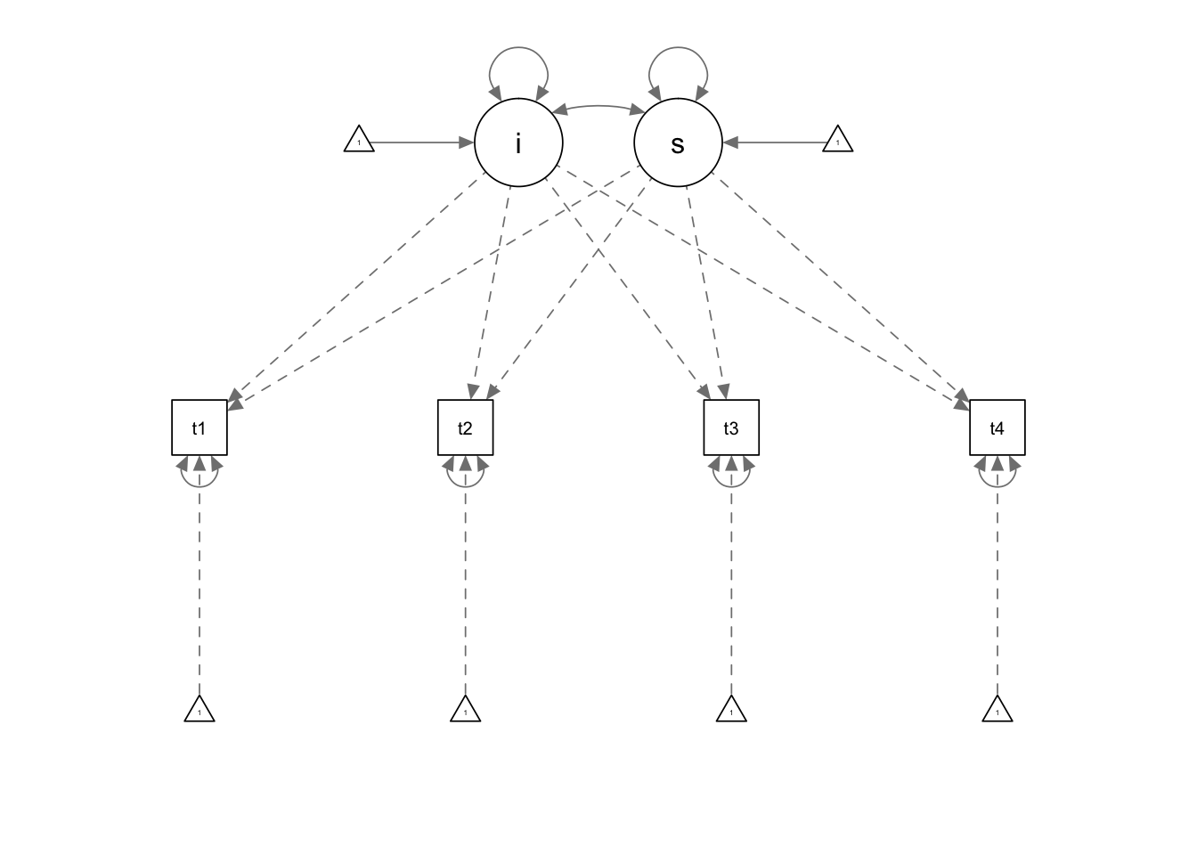
semPaths(fit.1, 'est')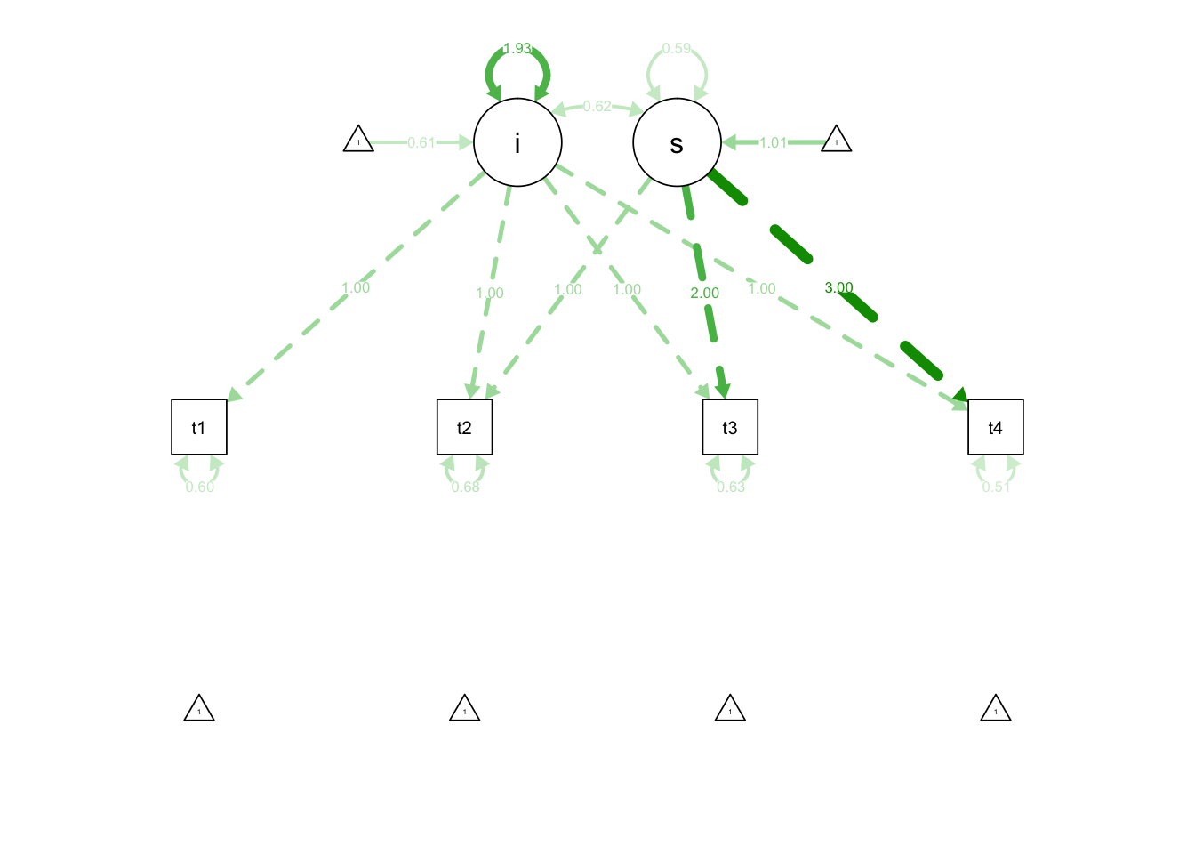
7.8.2 latent basis model
model.2 <- '  i =~ 1*t1 + 1*t2 + 1*t3 + 1*t4
            s =~ 0*t1 + t2 + t3 + 3*t4'
fit.2 <- growth(model.2, data=Demo.growth)
summary(fit.2)
## lavaan (0.5-23.1097) converged normally after 28 iterations
##
## Number of observations 400
##
## Estimator ML
## Minimum Function Test Statistic 6.447
## Degrees of freedom 3
## P-value (Chi-square) 0.092
##
## Parameter Estimates:
##
## Information Expected
## Standard Errors Standard
##
## Latent Variables:
## Estimate Std.Err z-value P(>|z|)
## i =~
## t1 1.000
## t2 1.000
## t3 1.000
## t4 1.000
## s =~
## t1 0.000
## t2 1.048 0.041 25.835 0.000
## t3 1.995 0.041 48.478 0.000
## t4 3.000
##
## Covariances:
## Estimate Std.Err z-value P(>|z|)
## i ~~
## s 0.610 0.072 8.483 0.000
##
## Intercepts:
## Estimate Std.Err z-value P(>|z|)
## .t1 0.000
## .t2 0.000
## .t3 0.000
## .t4 0.000
## i 0.597 0.078 7.625 0.000
## s 1.011 0.042 23.978 0.000
##
## Variances:
## Estimate Std.Err z-value P(>|z|)
## .t1 0.585 0.087 6.707 0.000
## .t2 0.675 0.061 11.072 0.000
## .t3 0.635 0.074 8.585 0.000
## .t4 0.514 0.131 3.941 0.000
## i 1.915 0.173 11.072 0.000
## s 0.593 0.053 11.210 0.000Does not change the fit of the model nor the implied means, but it can change your parameters by changing the time scaling.
7.8.3 constraining slope to be fixed only
model.3 <- '  i =~ 1*t1 + 1*t2 + 1*t3 + 1*t4
            s =~ 0*t1 + t2 + t3 + 3*t4

              s ~~0*s'
fit.3 <- growth(model.3, data=Demo.growth)
## Warning in lav_object_post_check(object): lavaan WARNING: covariance matrix of latent variables
## is not positive definite;
## use inspect(fit,"cov.lv") to investigate.summary(fit.3)## lavaan (0.5-23.1097) converged normally after 31 iterations
##
## Number of observations 400
##
## Estimator ML
## Minimum Function Test Statistic 303.366
## Degrees of freedom 4
## P-value (Chi-square) 0.000
##
## Parameter Estimates:
##
## Information Expected
## Standard Errors Standard
##
## Latent Variables:
## Estimate Std.Err z-value P(>|z|)
## i =~
## t1 1.000
## t2 1.000
## t3 1.000
## t4 1.000
## s =~
## t1 0.000
## t2 1.176 0.072 16.325 0.000
## t3 2.000 0.053 37.429 0.000
## t4 3.000
##
## Covariances:
## Estimate Std.Err z-value P(>|z|)
## i ~~
## s 0.949 0.070 13.511 0.000
##
## Intercepts:
## Estimate Std.Err z-value P(>|z|)
## .t1 0.000
## .t2 0.000
## .t3 0.000
## .t4 0.000
## i 0.528 0.088 5.986 0.000
## s 1.030 0.034 29.982 0.000
##
## Variances:
## Estimate Std.Err z-value P(>|z|)
## s 0.000
## .t1 2.618 0.177 14.770 0.000
## .t2 1.378 0.108 12.738 0.000
## .t3 0.439 0.079 5.567 0.000
## .t4 1.761 0.139 12.672 0.000
## i 0.662 0.200 3.302 0.0017.8.4 introducing covariates/predictors
# a linear growth model with a time invariatnt covariate

model.4 <- '
  # intercept and slope with fixed coefficients
    i =~ 1*t1 + 1*t2 + 1*t3 + 1*t4
    s =~ 0*t1 + 1*t2 + 2*t3 + 3*t4
  # regressions
    i ~ x1 + x2
    s ~ x1 + x2
'
fit.4 <- growth(model.4, data = Demo.growth)
summary(fit.4)
## lavaan (0.5-23.1097) converged normally after 31 iterations
##
## Number of observations 400
##
## Estimator ML
## Minimum Function Test Statistic 10.873
## Degrees of freedom 9
## P-value (Chi-square) 0.285
##
## Parameter Estimates:
##
## Information Expected
## Standard Errors Standard
##
## Latent Variables:
## Estimate Std.Err z-value P(>|z|)
## i =~
## t1 1.000
## t2 1.000
## t3 1.000
## t4 1.000
## s =~
## t1 0.000
## t2 1.000
## t3 2.000
## t4 3.000
##
## Regressions:
## Estimate Std.Err z-value P(>|z|)
## i ~
## x1 0.609 0.060 10.079 0.000
## x2 0.613 0.065 9.488 0.000
## s ~
## x1 0.263 0.029 9.157 0.000
## x2 0.517 0.031 16.868 0.000
##
## Covariances:
## Estimate Std.Err z-value P(>|z|)
## .i ~~
## .s 0.088 0.042 2.116 0.034
##
## Intercepts:
## Estimate Std.Err z-value P(>|z|)
## .t1 0.000
## .t2 0.000
## .t3 0.000
## .t4 0.000
## .i 0.586 0.062 9.400 0.000
## .s 0.958 0.030 32.382 0.000
##
## Variances:
## Estimate Std.Err z-value P(>|z|)
## .t1 0.597 0.085 7.067 0.000
## .t2 0.671 0.060 11.088 0.000
## .t3 0.599 0.065 9.254 0.000
## .t4 0.593 0.109 5.437 0.000
## .i 1.076 0.115 9.335 0.000
## .s 0.219 0.027 7.975 0.000# centered predictor
Demo.growth$x1.c <- scale(Demo.growth$x1, center=TRUE, scale = FALSE)
Demo.growth$x2.c <- scale(Demo.growth$x2, center=TRUE, scale = FALSE)
model.5 <- '
# intercept and slope with fixed coefficients
i =~ 1*t1 + 1*t2 + 1*t3 + 1*t4
s =~ 0*t1 + 1*t2 + 2*t3 + 3*t4
# regressions
i ~ x1.c + x2.c
s ~ x1.c + x2.c
'
fit.5 <- growth(model.5, data = Demo.growth)
summary(fit.5)## lavaan (0.5-23.1097) converged normally after 27 iterations
##
## Number of observations 400
##
## Estimator ML
## Minimum Function Test Statistic 10.873
## Degrees of freedom 9
## P-value (Chi-square) 0.285
##
## Parameter Estimates:
##
## Information Expected
## Standard Errors Standard
##
## Latent Variables:
## Estimate Std.Err z-value P(>|z|)
## i =~
## t1 1.000
## t2 1.000
## t3 1.000
## t4 1.000
## s =~
## t1 0.000
## t2 1.000
## t3 2.000
## t4 3.000
##
## Regressions:
## Estimate Std.Err z-value P(>|z|)
## i ~
## x1.c 0.609 0.060 10.079 0.000
## x2.c 0.613 0.065 9.488 0.000
## s ~
## x1.c 0.263 0.029 9.157 0.000
## x2.c 0.517 0.031 16.868 0.000
##
## Covariances:
## Estimate Std.Err z-value P(>|z|)
## .i ~~
## .s 0.088 0.042 2.116 0.034
##
## Intercepts:
## Estimate Std.Err z-value P(>|z|)
## .t1 0.000
## .t2 0.000
## .t3 0.000
## .t4 0.000
## .i 0.615 0.061 10.024 0.000
## .s 1.006 0.029 34.547 0.000
##
## Variances:
## Estimate Std.Err z-value P(>|z|)
## .t1 0.597 0.085 7.067 0.000
## .t2 0.671 0.060 11.088 0.000
## .t3 0.599 0.065 9.254 0.000
## .t4 0.593 0.109 5.437 0.000
## .i 1.076 0.115 9.335 0.000
## .s 0.219 0.027 7.975 0.000what is different what is the same?
7.8.5 introducing time varying covariates
# a linear growth model with a time-varying covariate
model.6 <- '
  # intercept and slope with fixed coefficients
    i =~ 1*t1 + 1*t2 + 1*t3 + 1*t4
    s =~ 0*t1 + 1*t2 + 2*t3 + 3*t4
  # regressions
    i ~ x1 + x2
    s ~ x1 + x2
  # time-varying covariates
    t1 ~ c1
    t2 ~ c2
    t3 ~ c3
    t4 ~ c4
'
fit.6 <- growth(model.6, data = Demo.growth)
summary(fit.6)
## lavaan (0.5-23.1097) converged normally after 31 iterations
##
## Number of observations 400
##
## Estimator ML
## Minimum Function Test Statistic 26.059
## Degrees of freedom 21
## P-value (Chi-square) 0.204
##
## Parameter Estimates:
##
## Information Expected
## Standard Errors Standard
##
## Latent Variables:
## Estimate Std.Err z-value P(>|z|)
## i =~
## t1 1.000
## t2 1.000
## t3 1.000
## t4 1.000
## s =~
## t1 0.000
## t2 1.000
## t3 2.000
## t4 3.000
##
## Regressions:
## Estimate Std.Err z-value P(>|z|)
## i ~
## x1 0.608 0.060 10.134 0.000
## x2 0.604 0.064 9.412 0.000
## s ~
## x1 0.262 0.029 9.198 0.000
## x2 0.522 0.031 17.083 0.000
## t1 ~
## c1 0.143 0.050 2.883 0.004
## t2 ~
## c2 0.289 0.046 6.295 0.000
## t3 ~
## c3 0.328 0.044 7.361 0.000
## t4 ~
## c4 0.330 0.058 5.655 0.000
##
## Covariances:
## Estimate Std.Err z-value P(>|z|)
## .i ~~
## .s 0.075 0.040 1.855 0.064
##
## Intercepts:
## Estimate Std.Err z-value P(>|z|)
## .t1 0.000
## .t2 0.000
## .t3 0.000
## .t4 0.000
## .i 0.580 0.062 9.368 0.000
## .s 0.958 0.029 32.552 0.000
##
## Variances:
## Estimate Std.Err z-value P(>|z|)
## .t1 0.580 0.080 7.230 0.000
## .t2 0.596 0.054 10.969 0.000
## .t3 0.481 0.055 8.745 0.000
## .t4 0.535 0.098 5.466 0.000
## .i 1.079 0.112 9.609 0.000
## .s 0.224 0.027 8.429 0.0007.8.6 multivariate growth curves
model.bi <- '
    #create positive affect growth model
    i.p =~ 1*PosAFF11 + 1*PosAFF12 + 1*PosAFF13
    s.p =~ 0*PosAFF11 + 1*PosAFF12 + 2*PosAFF13
# create negative affect growth model

   i.n =~ 1*NegAFF11 + 1*NegAFF12 + 1*NegAFF13
    s.n =~ 0*NegAFF11 + 1*NegAFF12 + 2*NegAFF13

'
fit.bi <- growth(model.bi, data = long)
## Warning in lav_object_post_check(object): lavaan WARNING: covariance matrix of latent variables
## is not positive definite;
## use inspect(fit,"cov.lv") to investigate.summary(fit.bi)## lavaan (0.5-23.1097) converged normally after 63 iterations
##
## Number of observations 368
##
## Estimator ML
## Minimum Function Test Statistic 56.908
## Degrees of freedom 7
## P-value (Chi-square) 0.000
##
## Parameter Estimates:
##
## Information Expected
## Standard Errors Standard
##
## Latent Variables:
## Estimate Std.Err z-value P(>|z|)
## i.p =~
## PosAFF11 1.000
## PosAFF12 1.000
## PosAFF13 1.000
## s.p =~
## PosAFF11 0.000
## PosAFF12 1.000
## PosAFF13 2.000
## i.n =~
## NegAFF11 1.000
## NegAFF12 1.000
## NegAFF13 1.000
## s.n =~
## NegAFF11 0.000
## NegAFF12 1.000
## NegAFF13 2.000
##
## Covariances:
## Estimate Std.Err z-value P(>|z|)
## i.p ~~
## s.p -0.033 0.025 -1.303 0.193
## i.n -0.127 0.021 -5.958 0.000
## s.n 0.047 0.012 3.793 0.000
## s.p ~~
## i.n 0.056 0.012 4.758 0.000
## s.n -0.036 0.007 -5.012 0.000
## i.n ~~
## s.n -0.032 0.018 -1.800 0.072
##
## Intercepts:
## Estimate Std.Err z-value P(>|z|)
## .PosAFF11 0.000
## .PosAFF12 0.000
## .PosAFF13 0.000
## .NegAFF11 0.000
## .NegAFF12 0.000
## .NegAFF13 0.000
## i.p 3.210 0.035 91.056 0.000
## s.p 0.045 0.020 2.269 0.023
## i.n 1.478 0.030 49.244 0.000
## s.n -0.036 0.018 -2.001 0.045
##
## Variances:
## Estimate Std.Err z-value P(>|z|)
## .PosAFF11 0.334 0.047 7.070 0.000
## .PosAFF12 0.235 0.023 10.407 0.000
## .PosAFF13 0.200 0.037 5.422 0.000
## .NegAFF11 0.289 0.034 8.562 0.000
## .NegAFF12 0.101 0.011 8.908 0.000
## .NegAFF13 0.157 0.023 6.735 0.000
## i.p 0.199 0.045 4.464 0.000
## s.p 0.016 0.020 0.791 0.429
## i.n 0.141 0.029 4.788 0.000
## s.n 0.012 0.014 0.861 0.389semPaths(fit.bi)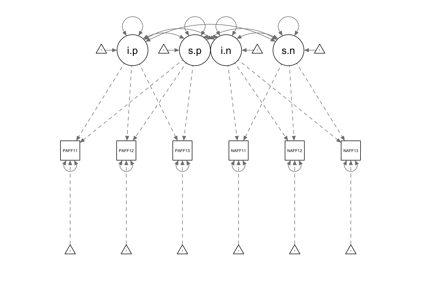
inspect(fit.bi,"cor.lv")## i.p s.p i.n s.n
## i.p 1.000
## s.p -0.577 1.000
## i.n -0.760 1.185 1.000
## s.n 0.947 -2.530 -0.760 1.000EEEEeeeee that is not good. What happened?
7.9 Measurement Invariance (MI)
To meaningfully look at means, we need to have the means mean the same thing. In other words, without using the word mean, we need to make sure that the measurment of the construct is consistent across time. If it isn’t, then what we may see as change actually reflect people responding to the indicators differently. For example, a common item on an extraversion scale is “Do you like to go to parties?” This is likely interpretted differently by a 20 year old compared to a 70 year old. This is due to what is normative, what parties look like that a typical 20 and 70 year old go to, etcetera. Another way to look at this is the item “2 x 3 = X, solve for X”. The reasons that a 8 year old and a 18 year old get the item incorrect is likely for different reasons (ie knowledge vs not being careful).
Maturation is the easiest way to see differences, but it also happens when you want to compare groups ie some anova design. This assumption is typically never critically examined.
7.9.1 types of MI
Configural (pattern). Typically always true with a decent measure of your construct. Can be tested through test statistics and eye-balling. Serves as default.
Weak (metric/loading). Can be easily met. Not meeting this shows big problems, unless you are working with a really large dataset (where there is large power to find differences).
Strong (Scalar/intercept). Need to meet this designation to run longitudinal models and look at means across time.
Strict (residual/error variance). Not necessarily better than Strong, and does not need to be satisfied to use longitudinal models. Why might this not hold even if you are assessing the same construct? Hint: think of what residual variance is made up of.
7.9.2 Testing MI
configural (baseline)
config <- '
## define latent variables
Pos1 =~ PosAFF11 + PosAFF21 + PosAFF31
Pos2 =~ PosAFF12 + PosAFF22 + PosAFF32
Pos3 =~ PosAFF13 + PosAFF23 + PosAFF33


## correlated residuals across time
PosAFF11 ~~ PosAFF12 + PosAFF13
PosAFF12 ~~ PosAFF13
PosAFF21 ~~ PosAFF22 + PosAFF23
PosAFF22 ~~ PosAFF23
PosAFF31 ~~ PosAFF32 + PosAFF33
PosAFF32 ~~ PosAFF33


'

config <- cfa(config, data=long, meanstructure=TRUE, std.lv=TRUE)

summary(config, standardized=TRUE, fit.measures=TRUE)
## lavaan (0.5-23.1097) converged normally after 72 iterations
##
## Number of observations 368
##
## Estimator ML
## Minimum Function Test Statistic 9.266
## Degrees of freedom 15
## P-value (Chi-square) 0.863
##
## Model test baseline model:
##
## Minimum Function Test Statistic 2688.088
## Degrees of freedom 36
## P-value 0.000
##
## User model versus baseline model:
##
## Comparative Fit Index (CFI) 1.000
## Tucker-Lewis Index (TLI) 1.005
##
## Loglikelihood and Information Criteria:
##
## Loglikelihood user model (H0) -2040.957
## Loglikelihood unrestricted model (H1) -2036.324
##
## Number of free parameters 39
## Akaike (AIC) 4159.914
## Bayesian (BIC) 4312.329
## Sample-size adjusted Bayesian (BIC) 4188.596
##
## Root Mean Square Error of Approximation:
##
## RMSEA 0.000
## 90 Percent Confidence Interval 0.000 0.026
## P-value RMSEA <= 0.05 0.997
##
## Standardized Root Mean Square Residual:
##
## SRMR 0.011
##
## Parameter Estimates:
##
## Information Expected
## Standard Errors Standard
##
## Latent Variables:
## Estimate Std.Err z-value P(>|z|) Std.lv Std.all
## Pos1 =~
## PosAFF11 0.656 0.030 22.030 0.000 0.656 0.906
## PosAFF21 0.652 0.031 20.908 0.000 0.652 0.877
## PosAFF31 0.682 0.031 22.157 0.000 0.682 0.908
## Pos2 =~
## PosAFF12 0.555 0.026 21.138 0.000 0.555 0.881
## PosAFF22 0.643 0.030 21.651 0.000 0.643 0.894
## PosAFF32 0.642 0.027 23.348 0.000 0.642 0.936
## Pos3 =~
## PosAFF13 0.509 0.024 21.036 0.000 0.509 0.888
## PosAFF23 0.545 0.027 20.347 0.000 0.545 0.867
## PosAFF33 0.537 0.026 20.763 0.000 0.537 0.878
##
## Covariances:
## Estimate Std.Err z-value P(>|z|) Std.lv Std.all
## .PosAFF11 ~~
## .PosAFF12 0.002 0.007 0.325 0.745 0.002 0.024
## .PosAFF13 0.001 0.007 0.207 0.836 0.001 0.017
## .PosAFF12 ~~
## .PosAFF13 0.003 0.006 0.517 0.605 0.003 0.039
## .PosAFF21 ~~
## .PosAFF22 0.006 0.008 0.784 0.433 0.006 0.056
## .PosAFF23 0.006 0.008 0.773 0.439 0.006 0.055
## .PosAFF22 ~~
## .PosAFF23 0.011 0.007 1.525 0.127 0.011 0.111
## .PosAFF31 ~~
## .PosAFF32 0.008 0.007 1.097 0.273 0.008 0.100
## .PosAFF33 0.016 0.007 2.215 0.027 0.016 0.177
## .PosAFF32 ~~
## .PosAFF33 0.005 0.006 0.773 0.440 0.005 0.068
## Pos1 ~~
## Pos2 0.471 0.044 10.609 0.000 0.471 0.471
## Pos3 0.399 0.048 8.226 0.000 0.399 0.399
## Pos2 ~~
## Pos3 0.450 0.046 9.806 0.000 0.450 0.450
##
## Intercepts:
## Estimate Std.Err z-value P(>|z|) Std.lv Std.all
## .PosAFF11 3.212 0.038 85.122 0.000 3.212 4.437
## .PosAFF21 3.105 0.039 80.035 0.000 3.105 4.172
## .PosAFF31 3.248 0.039 82.962 0.000 3.248 4.325
## .PosAFF12 3.253 0.033 99.116 0.000 3.253 5.167
## .PosAFF22 3.126 0.037 83.356 0.000 3.126 4.345
## .PosAFF32 3.274 0.036 91.602 0.000 3.274 4.775
## .PosAFF13 3.302 0.030 110.504 0.000 3.302 5.760
## .PosAFF23 3.094 0.033 94.403 0.000 3.094 4.921
## .PosAFF33 3.280 0.032 102.942 0.000 3.280 5.366
## Pos1 0.000 0.000 0.000
## Pos2 0.000 0.000 0.000
## Pos3 0.000 0.000 0.000
##
## Variances:
## Estimate Std.Err z-value P(>|z|) Std.lv Std.all
## .PosAFF11 0.093 0.011 8.155 0.000 0.093 0.178
## .PosAFF21 0.128 0.013 9.770 0.000 0.128 0.231
## .PosAFF31 0.099 0.012 8.092 0.000 0.099 0.176
## .PosAFF12 0.089 0.009 9.942 0.000 0.089 0.224
## .PosAFF22 0.104 0.011 9.363 0.000 0.104 0.202
## .PosAFF32 0.058 0.009 6.467 0.000 0.058 0.124
## .PosAFF13 0.070 0.008 8.211 0.000 0.070 0.212
## .PosAFF23 0.098 0.011 9.234 0.000 0.098 0.248
## .PosAFF33 0.086 0.010 8.719 0.000 0.086 0.229
## Pos1 1.000 1.000 1.000
## Pos2 1.000 1.000 1.000
## Pos3 1.000 1.000 1.000weak (constrain loadings)
weak <- '
## define latent variables
Pos1 =~ L1*PosAFF11 + L2*PosAFF21 + L3*PosAFF31
Pos2 =~ L1*PosAFF12 + L2*PosAFF22 + L3*PosAFF32
Pos3 =~ L1*PosAFF13 + L2*PosAFF23 + L3*PosAFF33


## free latent variances at later times (only set the scale once)
Pos2 ~~ NA*Pos2
Pos3 ~~ NA*Pos3

## correlated residuals across time
PosAFF11 ~~ PosAFF12 + PosAFF13
PosAFF12 ~~ PosAFF13
PosAFF21 ~~ PosAFF22 + PosAFF23
PosAFF22 ~~ PosAFF23
PosAFF31 ~~ PosAFF32 + PosAFF33
PosAFF32 ~~ PosAFF33


'

weak <- cfa(weak, data=long, meanstructure=TRUE, std.lv=TRUE)

summary(weak, standardized=TRUE, fit.measures=TRUE)
## lavaan (0.5-23.1097) converged normally after 81 iterations
##
## Number of observations 368
##
## Estimator ML
## Minimum Function Test Statistic 17.684
## Degrees of freedom 19
## P-value (Chi-square) 0.544
##
## Model test baseline model:
##
## Minimum Function Test Statistic 2688.088
## Degrees of freedom 36
## P-value 0.000
##
## User model versus baseline model:
##
## Comparative Fit Index (CFI) 1.000
## Tucker-Lewis Index (TLI) 1.001
##
## Loglikelihood and Information Criteria:
##
## Loglikelihood user model (H0) -2045.166
## Loglikelihood unrestricted model (H1) -2036.324
##
## Number of free parameters 35
## Akaike (AIC) 4160.332
## Bayesian (BIC) 4297.114
## Sample-size adjusted Bayesian (BIC) 4186.072
##
## Root Mean Square Error of Approximation:
##
## RMSEA 0.000
## 90 Percent Confidence Interval 0.000 0.042
## P-value RMSEA <= 0.05 0.983
##
## Standardized Root Mean Square Residual:
##
## SRMR 0.021
##
## Parameter Estimates:
##
## Information Expected
## Standard Errors Standard
##
## Latent Variables:
## Estimate Std.Err z-value P(>|z|) Std.lv Std.all
## Pos1 =~
## PosAFF11 (L1) 0.631 0.027 23.651 0.000 0.631 0.894
## PosAFF21 (L2) 0.677 0.029 23.460 0.000 0.677 0.887
## PosAFF31 (L3) 0.686 0.029 23.837 0.000 0.686 0.910
## Pos2 =~
## PosAFF12 (L1) 0.631 0.027 23.651 0.000 0.582 0.894
## PosAFF22 (L2) 0.677 0.029 23.460 0.000 0.625 0.886
## PosAFF32 (L3) 0.686 0.029 23.837 0.000 0.633 0.931
## Pos3 =~
## PosAFF13 (L1) 0.631 0.027 23.651 0.000 0.503 0.883
## PosAFF23 (L2) 0.677 0.029 23.460 0.000 0.540 0.864
## PosAFF33 (L3) 0.686 0.029 23.837 0.000 0.547 0.885
##
## Covariances:
## Estimate Std.Err z-value P(>|z|) Std.lv Std.all
## .PosAFF11 ~~
## .PosAFF12 0.003 0.007 0.395 0.693 0.003 0.029
## .PosAFF13 0.002 0.007 0.231 0.817 0.002 0.018
## .PosAFF12 ~~
## .PosAFF13 0.002 0.006 0.404 0.686 0.002 0.031
## .PosAFF21 ~~
## .PosAFF22 0.006 0.008 0.676 0.499 0.006 0.049
## .PosAFF23 0.005 0.008 0.646 0.518 0.005 0.047
## .PosAFF22 ~~
## .PosAFF23 0.012 0.007 1.598 0.110 0.012 0.114
## .PosAFF31 ~~
## .PosAFF32 0.008 0.007 1.185 0.236 0.008 0.107
## .PosAFF33 0.016 0.007 2.214 0.027 0.016 0.182
## .PosAFF32 ~~
## .PosAFF33 0.005 0.006 0.766 0.444 0.005 0.067
## Pos1 ~~
## Pos2 0.437 0.046 9.404 0.000 0.474 0.474
## Pos3 0.319 0.042 7.578 0.000 0.400 0.400
## Pos2 ~~
## Pos3 0.332 0.047 7.030 0.000 0.450 0.450
##
## Intercepts:
## Estimate Std.Err z-value P(>|z|) Std.lv Std.all
## .PosAFF11 3.212 0.037 87.342 0.000 3.212 4.553
## .PosAFF21 3.105 0.040 78.061 0.000 3.105 4.069
## .PosAFF31 3.248 0.039 82.691 0.000 3.248 4.311
## .PosAFF12 3.253 0.034 95.798 0.000 3.253 4.994
## .PosAFF22 3.126 0.037 85.004 0.000 3.126 4.431
## .PosAFF32 3.274 0.035 92.400 0.000 3.274 4.817
## .PosAFF13 3.302 0.030 111.238 0.000 3.302 5.799
## .PosAFF23 3.094 0.033 94.971 0.000 3.094 4.951
## .PosAFF33 3.280 0.032 101.745 0.000 3.280 5.304
## Pos1 0.000 0.000 0.000
## Pos2 0.000 0.000 0.000
## Pos3 0.000 0.000 0.000
##
## Variances:
## Estimate Std.Err z-value P(>|z|) Std.lv Std.all
## Pos2 0.853 0.086 9.942 0.000 1.000 1.000
## Pos3 0.636 0.067 9.479 0.000 1.000 1.000
## .PosAFF11 0.100 0.011 9.159 0.000 0.100 0.201
## .PosAFF21 0.124 0.013 9.501 0.000 0.124 0.213
## .PosAFF31 0.098 0.012 8.261 0.000 0.098 0.172
## .PosAFF12 0.085 0.009 9.548 0.000 0.085 0.201
## .PosAFF22 0.107 0.011 9.929 0.000 0.107 0.215
## .PosAFF32 0.061 0.009 7.123 0.000 0.061 0.132
## .PosAFF13 0.071 0.008 8.812 0.000 0.071 0.219
## .PosAFF23 0.099 0.010 9.680 0.000 0.099 0.254
## .PosAFF33 0.083 0.009 8.776 0.000 0.083 0.218
## Pos1 1.000 1.000 1.000Strong (constrain loadings and intercepts)
strong <- '
## define latent variables
Pos1 =~ L1*PosAFF11 + L2*PosAFF21 + L3*PosAFF31
Pos2 =~ L1*PosAFF12 + L2*PosAFF22 + L3*PosAFF32
Pos3 =~ L1*PosAFF13 + L2*PosAFF23 + L3*PosAFF33


## free latent variances at later times (only set the scale once)
Pos2 ~~ NA*Pos2
Pos3 ~~ NA*Pos3


## correlated residuals across time
PosAFF11 ~~ PosAFF12 + PosAFF13
PosAFF12 ~~ PosAFF13
PosAFF21 ~~ PosAFF22 + PosAFF23
PosAFF22 ~~ PosAFF23
PosAFF31 ~~ PosAFF32 + PosAFF33
PosAFF32 ~~ PosAFF33


## constrain intercepts across time
PosAFF11 ~ t1*1
PosAFF21 ~ t2*1
PosAFF31 ~ t3*1


PosAFF12 ~ t1*1
PosAFF22 ~ t2*1
PosAFF32 ~ t3*1


PosAFF13 ~ t1*1
PosAFF23 ~ t2*1
PosAFF33 ~ t3*1


## free latent means at later times (only set the scale once)
Pos2 ~ NA*1
Pos3 ~ NA*1'

strong <- cfa(strong, data=long, meanstructure=TRUE, std.lv=TRUE)

summary(strong, standardized=TRUE, fit.measures=TRUE)
## lavaan (0.5-23.1097) converged normally after 81 iterations
##
## Number of observations 368
##
## Estimator ML
## Minimum Function Test Statistic 30.144
## Degrees of freedom 23
## P-value (Chi-square) 0.145
##
## Model test baseline model:
##
## Minimum Function Test Statistic 2688.088
## Degrees of freedom 36
## P-value 0.000
##
## User model versus baseline model:
##
## Comparative Fit Index (CFI) 0.997
## Tucker-Lewis Index (TLI) 0.996
##
## Loglikelihood and Information Criteria:
##
## Loglikelihood user model (H0) -2051.396
## Loglikelihood unrestricted model (H1) -2036.324
##
## Number of free parameters 31
## Akaike (AIC) 4164.792
## Bayesian (BIC) 4285.943
## Sample-size adjusted Bayesian (BIC) 4187.591
##
## Root Mean Square Error of Approximation:
##
## RMSEA 0.029
## 90 Percent Confidence Interval 0.000 0.055
## P-value RMSEA <= 0.05 0.901
##
## Standardized Root Mean Square Residual:
##
## SRMR 0.024
##
## Parameter Estimates:
##
## Information Expected
## Standard Errors Standard
##
## Latent Variables:
## Estimate Std.Err z-value P(>|z|) Std.lv Std.all
## Pos1 =~
## PosAFF11 (L1) 0.631 0.027 23.635 0.000 0.631 0.893
## PosAFF21 (L2) 0.676 0.029 23.441 0.000 0.676 0.886
## PosAFF31 (L3) 0.686 0.029 23.838 0.000 0.686 0.910
## Pos2 =~
## PosAFF12 (L1) 0.631 0.027 23.635 0.000 0.582 0.894
## PosAFF22 (L2) 0.676 0.029 23.441 0.000 0.624 0.886
## PosAFF32 (L3) 0.686 0.029 23.838 0.000 0.633 0.932
## Pos3 =~
## PosAFF13 (L1) 0.631 0.027 23.635 0.000 0.503 0.882
## PosAFF23 (L2) 0.676 0.029 23.441 0.000 0.539 0.862
## PosAFF33 (L3) 0.686 0.029 23.838 0.000 0.547 0.885
##
## Covariances:
## Estimate Std.Err z-value P(>|z|) Std.lv Std.all
## .PosAFF11 ~~
## .PosAFF12 0.003 0.007 0.471 0.638 0.003 0.035
## .PosAFF13 0.000 0.007 0.030 0.976 0.000 0.002
## .PosAFF12 ~~
## .PosAFF13 0.002 0.006 0.299 0.765 0.002 0.023
## .PosAFF21 ~~
## .PosAFF22 0.006 0.008 0.718 0.473 0.006 0.051
## .PosAFF23 0.004 0.008 0.521 0.602 0.004 0.038
## .PosAFF22 ~~
## .PosAFF23 0.011 0.007 1.530 0.126 0.011 0.109
## .PosAFF31 ~~
## .PosAFF32 0.008 0.007 1.160 0.246 0.008 0.105
## .PosAFF33 0.017 0.007 2.261 0.024 0.017 0.187
## .PosAFF32 ~~
## .PosAFF33 0.005 0.006 0.795 0.427 0.005 0.070
## Pos1 ~~
## Pos2 0.438 0.047 9.409 0.000 0.474 0.474
## Pos3 0.320 0.042 7.590 0.000 0.401 0.401
## Pos2 ~~
## Pos3 0.332 0.047 7.027 0.000 0.450 0.450
##
## Intercepts:
## Estimate Std.Err z-value P(>|z|) Std.lv Std.all
## .PosAFF11 (t1) 3.237 0.035 92.743 0.000 3.237 4.583
## .PosAFF21 (t2) 3.084 0.038 81.945 0.000 3.084 4.043
## .PosAFF31 (t3) 3.244 0.038 85.408 0.000 3.244 4.304
## .PosAFF12 (t1) 3.237 0.035 92.743 0.000 3.237 4.967
## .PosAFF22 (t2) 3.084 0.038 81.945 0.000 3.084 4.375
## .PosAFF32 (t3) 3.244 0.038 85.408 0.000 3.244 4.771
## .PosAFF13 (t1) 3.237 0.035 92.743 0.000 3.237 5.674
## .PosAFF23 (t2) 3.084 0.038 81.945 0.000 3.084 4.931
## .PosAFF33 (t3) 3.244 0.038 85.408 0.000 3.244 5.249
## Pos2 0.044 0.055 0.798 0.425 0.047 0.047
## Pos3 0.058 0.055 1.043 0.297 0.072 0.072
## Pos1 0.000 0.000 0.000
##
## Variances:
## Estimate Std.Err z-value P(>|z|) Std.lv Std.all
## Pos2 0.853 0.086 9.942 0.000 1.000 1.000
## Pos3 0.636 0.067 9.475 0.000 1.000 1.000
## .PosAFF11 0.101 0.011 9.188 0.000 0.101 0.203
## .PosAFF21 0.125 0.013 9.527 0.000 0.125 0.215
## .PosAFF31 0.097 0.012 8.216 0.000 0.097 0.172
## .PosAFF12 0.086 0.009 9.551 0.000 0.086 0.201
## .PosAFF22 0.107 0.011 9.947 0.000 0.107 0.216
## .PosAFF32 0.061 0.009 7.094 0.000 0.061 0.132
## .PosAFF13 0.073 0.008 8.865 0.000 0.073 0.223
## .PosAFF23 0.101 0.010 9.725 0.000 0.101 0.257
## .PosAFF33 0.083 0.009 8.706 0.000 0.083 0.216
## Pos1 1.000 1.000 1.000Strict (loadings, intercept, residual variances)
strict <- '
## define latent variables
Pos1 =~ L1*PosAFF11 + L2*PosAFF21 + L3*PosAFF31
Pos2 =~ L1*PosAFF12 + L2*PosAFF22 + L3*PosAFF32
Pos3 =~ L1*PosAFF13 + L2*PosAFF23 + L3*PosAFF33


## free latent variances at later times (only set the scale once)
Pos2 ~~ NA*Pos2
Pos3 ~~ NA*Pos3


## correlated residuals across time
PosAFF11 ~~ PosAFF12 + PosAFF13
PosAFF12 ~~ PosAFF13
PosAFF21 ~~ PosAFF22 + PosAFF23
PosAFF22 ~~ PosAFF23
PosAFF31 ~~ PosAFF32 + PosAFF33
PosAFF32 ~~ PosAFF33

## equality of residuals
PosAFF11 ~~ r*PosAFF11
PosAFF12 ~~ r*PosAFF12
PosAFF13 ~~ r*PosAFF13

PosAFF21 ~~ r*PosAFF21
PosAFF22 ~~ r*PosAFF22
PosAFF23 ~~ r*PosAFF23

PosAFF31 ~~ r*PosAFF31
PosAFF32 ~~ r*PosAFF32
PosAFF33 ~~ r*PosAFF33


## constrain intercepts across time
PosAFF11 ~ t1*1
PosAFF21 ~ t2*1
PosAFF31 ~ t3*1


PosAFF12 ~ t1*1
PosAFF22 ~ t2*1
PosAFF32 ~ t3*1


PosAFF13 ~ t1*1
PosAFF23 ~ t2*1
PosAFF33 ~ t3*1


## free latent means at later times (only set the scale once)
Pos2 ~ NA*1
Pos3 ~ NA*1'

strict <- cfa(strict, data=long, meanstructure=TRUE, std.lv=TRUE)

summary(strict, standardized=TRUE, fit.measures=TRUE)
## lavaan (0.5-23.1097) converged normally after 85 iterations
##
## Number of observations 368
##
## Estimator ML
## Minimum Function Test Statistic 60.491
## Degrees of freedom 31
## P-value (Chi-square) 0.001
##
## Model test baseline model:
##
## Minimum Function Test Statistic 2688.088
## Degrees of freedom 36
## P-value 0.000
##
## User model versus baseline model:
##
## Comparative Fit Index (CFI) 0.989
## Tucker-Lewis Index (TLI) 0.987
##
## Loglikelihood and Information Criteria:
##
## Loglikelihood user model (H0) -2066.569
## Loglikelihood unrestricted model (H1) -2036.324
##
## Number of free parameters 23
## Akaike (AIC) 4179.139
## Bayesian (BIC) 4269.025
## Sample-size adjusted Bayesian (BIC) 4196.054
##
## Root Mean Square Error of Approximation:
##
## RMSEA 0.051
## 90 Percent Confidence Interval 0.031 0.070
## P-value RMSEA <= 0.05 0.445
##
## Standardized Root Mean Square Residual:
##
## SRMR 0.026
##
## Parameter Estimates:
##
## Information Expected
## Standard Errors Standard
##
## Latent Variables:
## Estimate Std.Err z-value P(>|z|) Std.lv Std.all
## Pos1 =~
## PosAFF11 (L1) 0.631 0.026 23.891 0.000 0.631 0.901
## PosAFF21 (L2) 0.689 0.028 24.210 0.000 0.689 0.915
## PosAFF31 (L3) 0.680 0.028 24.061 0.000 0.680 0.913
## Pos2 =~
## PosAFF12 (L1) 0.631 0.026 23.891 0.000 0.579 0.885
## PosAFF22 (L2) 0.689 0.028 24.210 0.000 0.632 0.901
## PosAFF32 (L3) 0.680 0.028 24.061 0.000 0.623 0.899
## Pos3 =~
## PosAFF13 (L1) 0.631 0.026 23.891 0.000 0.500 0.854
## PosAFF23 (L2) 0.689 0.028 24.210 0.000 0.545 0.873
## PosAFF33 (L3) 0.680 0.028 24.061 0.000 0.538 0.871
##
## Covariances:
## Estimate Std.Err z-value P(>|z|) Std.lv Std.all
## .PosAFF11 ~~
## .PosAFF12 0.004 0.007 0.617 0.537 0.004 0.045
## .PosAFF13 0.002 0.007 0.280 0.780 0.002 0.020
## .PosAFF12 ~~
## .PosAFF13 0.003 0.007 0.394 0.693 0.003 0.029
## .PosAFF21 ~~
## .PosAFF22 0.003 0.007 0.346 0.730 0.003 0.027
## .PosAFF23 0.002 0.007 0.228 0.820 0.002 0.018
## .PosAFF22 ~~
## .PosAFF23 0.009 0.007 1.259 0.208 0.009 0.098
## .PosAFF31 ~~
## .PosAFF32 0.011 0.007 1.508 0.132 0.011 0.117
## .PosAFF33 0.016 0.007 2.310 0.021 0.016 0.177
## .PosAFF32 ~~
## .PosAFF33 0.008 0.007 1.186 0.236 0.008 0.091
## Pos1 ~~
## Pos2 0.433 0.046 9.372 0.000 0.472 0.472
## Pos3 0.318 0.042 7.613 0.000 0.402 0.402
## Pos2 ~~
## Pos3 0.330 0.047 7.031 0.000 0.454 0.454
##
## Intercepts:
## Estimate Std.Err z-value P(>|z|) Std.lv Std.all
## .PosAFF11 (t1) 3.236 0.035 92.686 0.000 3.236 4.617
## .PosAFF21 (t2) 3.087 0.038 81.529 0.000 3.087 4.100
## .PosAFF31 (t3) 3.245 0.038 86.233 0.000 3.245 4.359
## .PosAFF12 (t1) 3.236 0.035 92.686 0.000 3.236 4.947
## .PosAFF22 (t2) 3.087 0.038 81.529 0.000 3.087 4.402
## .PosAFF32 (t3) 3.245 0.038 86.233 0.000 3.245 4.679
## .PosAFF13 (t1) 3.236 0.035 92.686 0.000 3.236 5.530
## .PosAFF23 (t2) 3.087 0.038 81.529 0.000 3.087 4.944
## .PosAFF33 (t3) 3.245 0.038 86.233 0.000 3.245 5.251
## Pos2 0.044 0.055 0.799 0.424 0.048 0.048
## Pos3 0.052 0.055 0.945 0.345 0.066 0.066
## Pos1 0.000 0.000 0.000
##
## Variances:
## Estimate Std.Err z-value P(>|z|) Std.lv Std.all
## Pos2 0.841 0.085 9.950 0.000 1.000 1.000
## Pos3 0.627 0.066 9.494 0.000 1.000 1.000
## .PosAFF11 (r) 0.093 0.003 33.038 0.000 0.093 0.188
## .PosAFF12 (r) 0.093 0.003 33.038 0.000 0.093 0.216
## .PosAFF13 (r) 0.093 0.003 33.038 0.000 0.093 0.270
## .PosAFF21 (r) 0.093 0.003 33.038 0.000 0.093 0.163
## .PosAFF22 (r) 0.093 0.003 33.038 0.000 0.093 0.188
## .PosAFF23 (r) 0.093 0.003 33.038 0.000 0.093 0.237
## .PosAFF31 (r) 0.093 0.003 33.038 0.000 0.093 0.167
## .PosAFF32 (r) 0.093 0.003 33.038 0.000 0.093 0.192
## .PosAFF33 (r) 0.093 0.003 33.038 0.000 0.093 0.242
## Pos1 1.000 1.000 1.000Note that there are other types of MI that we could investigate, depending on what we are interested in. We could look at equality of latent means and variances, as well as regressions, if they were in the model.
7.9.3 Comparing the models
Usually done through chi-square difference test. But this is a very sensitive test, especially with larger samples. Better to look at changes in CFI. If delta is .01 or greater than maybe it shows misfit.
##Compare configural and weak model
anova(config, weak)
## Chi Square Difference Test
##
## Df AIC BIC Chisq Chisq diff Df diff Pr(>Chisq)
## config 15 4159.9 4312.3 9.2658
## weak 19 4160.3 4297.1 17.6836 8.4179 4 0.07742 .
## ---
## Signif. codes: 0 '***' 0.001 '**' 0.01 '*' 0.05 '.' 0.1 ' ' 1##Compare weak and strong model
anova(weak, strong)## Chi Square Difference Test
##
## Df AIC BIC Chisq Chisq diff Df diff Pr(>Chisq)
## weak 19 4160.3 4297.1 17.684
## strong 23 4164.8 4285.9 30.144 12.461 4 0.01424 *
## ---
## Signif. codes: 0 '***' 0.001 '**' 0.01 '*' 0.05 '.' 0.1 ' ' 1fitmeasures(weak)['cfi']## cfi
## 1fitmeasures(strong)['cfi']## cfi
## 0.9973062fitmeasures(strict)['cfi']## cfi
## 0.98888017.10 Second order growth model
Repeated measures are latent. Why would we want to do this?
sec.order <- '
## define latent variables
Pos1 =~ NA*PosAFF11 + L1*PosAFF11 + L2*PosAFF21 + L3*PosAFF31
Pos2 =~ NA*PosAFF12 + L1*PosAFF12 + L2*PosAFF22 + L3*PosAFF32
Pos3 =~ NA*PosAFF13 + L1*PosAFF13 + L2*PosAFF23 + L3*PosAFF33

## intercepts
PosAFF11 ~ t1*1
PosAFF21 ~ t2*1
PosAFF31 ~ t3*1

PosAFF12 ~ t1*1
PosAFF22 ~ t2*1
PosAFF32 ~ t3*1

PosAFF13 ~ t1*1
PosAFF23 ~ t2*1
PosAFF33 ~ t3*1


## correlated residuals across time
PosAFF11 ~~ PosAFF12 + PosAFF13
PosAFF12 ~~ PosAFF13
PosAFF21 ~~ PosAFF22 + PosAFF23
PosAFF22 ~~ PosAFF23
PosAFF31 ~~ PosAFF32 + PosAFF33
PosAFF32 ~~ PosAFF33


## latent variable intercepts
Pos1 ~ 0*1
Pos2  ~ 0*1
Pos3  ~ 0*1

#model constraints for effect coding
## loadings must average to 1
L1 == 3 - L2 - L3
## means must average to 0
t1 == 0 - t2 - t3

i =~ 1*Pos1 + 1*Pos2 + 1*Pos3
s =~ 0*Pos1 + 1*Pos2 + 2*Pos3 '


fit.sec.order <- growth(sec.order, data=long, missing = "ML")
summary(fit.sec.order, fit.measures=TRUE)
## lavaan (0.5-23.1097) converged normally after 99 iterations
##
## Number of observations 368
##
## Number of missing patterns 1
##
## Estimator ML
## Minimum Function Test Statistic 30.254
## Degrees of freedom 24
## P-value (Chi-square) 0.176
##
## Model test baseline model:
##
## Minimum Function Test Statistic 2688.088
## Degrees of freedom 36
## P-value 0.000
##
## User model versus baseline model:
##
## Comparative Fit Index (CFI) 0.998
## Tucker-Lewis Index (TLI) 0.996
##
## Loglikelihood and Information Criteria:
##
## Loglikelihood user model (H0) -2051.451
## Loglikelihood unrestricted model (H1) -2036.324
##
## Number of free parameters 30
## Akaike (AIC) 4162.902
## Bayesian (BIC) 4280.145
## Sample-size adjusted Bayesian (BIC) 4184.966
##
## Root Mean Square Error of Approximation:
##
## RMSEA 0.027
## 90 Percent Confidence Interval 0.000 0.053
## P-value RMSEA <= 0.05 0.926
##
## Standardized Root Mean Square Residual:
##
## SRMR 0.025
##
## Parameter Estimates:
##
## Information Observed
## Standard Errors Standard
##
## Latent Variables:
## Estimate Std.Err z-value P(>|z|)
## Pos1 =~
## PosAFF11 (L1) 0.950 0.014 68.551 0.000
## PosAFF21 (L2) 1.018 0.015 69.038 0.000
## PosAFF31 (L3) 1.033 0.014 73.342 0.000
## Pos2 =~
## PosAFF12 (L1) 0.950 0.014 68.551 0.000
## PosAFF22 (L2) 1.018 0.015 69.038 0.000
## PosAFF32 (L3) 1.033 0.014 73.342 0.000
## Pos3 =~
## PosAFF13 (L1) 0.950 0.014 68.551 0.000
## PosAFF23 (L2) 1.018 0.015 69.038 0.000
## PosAFF33 (L3) 1.033 0.014 73.342 0.000
## i =~
## Pos1 1.000
## Pos2 1.000
## Pos3 1.000
## s =~
## Pos1 0.000
## Pos2 1.000
## Pos3 2.000
##
## Covariances:
## Estimate Std.Err z-value P(>|z|)
## .PosAFF11 ~~
## .PosAFF12 0.003 0.007 0.465 0.642
## .PosAFF13 0.000 0.007 0.029 0.977
## .PosAFF12 ~~
## .PosAFF13 0.002 0.006 0.306 0.759
## .PosAFF21 ~~
## .PosAFF22 0.006 0.008 0.716 0.474
## .PosAFF23 0.004 0.008 0.520 0.603
## .PosAFF22 ~~
## .PosAFF23 0.011 0.007 1.518 0.129
## .PosAFF31 ~~
## .PosAFF32 0.008 0.007 1.159 0.247
## .PosAFF33 0.017 0.007 2.253 0.024
## .PosAFF32 ~~
## .PosAFF33 0.005 0.006 0.791 0.429
## i ~~
## s -0.052 0.023 -2.216 0.027
##
## Intercepts:
## Estimate Std.Err z-value P(>|z|)
## .PosAFF11 (t1) 0.210 0.045 4.645 0.000
## .PosAFF21 (t2) -0.161 0.048 -3.344 0.001
## .PosAFF31 (t3) -0.049 0.046 -1.067 0.286
## .PosAFF12 (t1) 0.210 0.045 4.645 0.000
## .PosAFF22 (t2) -0.161 0.048 -3.344 0.001
## .PosAFF32 (t3) -0.049 0.046 -1.067 0.286
## .PosAFF13 (t1) 0.210 0.045 4.645 0.000
## .PosAFF23 (t2) -0.161 0.048 -3.344 0.001
## .PosAFF33 (t3) -0.049 0.046 -1.067 0.286
## Pos1 0.000
## Pos2 0.000
## Pos3 0.000
## i 3.192 0.034 92.584 0.000
## s 0.019 0.018 1.016 0.310
##
## Variances:
## Estimate Std.Err z-value P(>|z|)
## .PosAFF11 0.101 0.011 9.101 0.000
## .PosAFF21 0.125 0.013 9.479 0.000
## .PosAFF31 0.097 0.012 8.170 0.000
## .PosAFF12 0.086 0.009 9.536 0.000
## .PosAFF22 0.107 0.011 9.917 0.000
## .PosAFF32 0.061 0.009 7.052 0.000
## .PosAFF13 0.072 0.008 8.770 0.000
## .PosAFF23 0.101 0.010 9.655 0.000
## .PosAFF33 0.083 0.009 8.716 0.000
## Pos1 0.196 0.043 4.553 0.000
## Pos2 0.207 0.023 9.132 0.000
## Pos3 0.129 0.034 3.767 0.000
## i 0.245 0.044 5.627 0.000
## s 0.029 0.019 1.542 0.123
##
## Constraints:
## |Slack|
## L1 - (3-L2-L3) 0.000
## t1 - (0-t2-t3) 0.0007.11 Multple groups
group <- read_csv("~/Box Sync/5165 Applied Longitudinal Data Analysis/Longitudinal/group.csv")## Parsed with column specification:
## cols(
## P1 = col_double(),
## P2 = col_double(),
## P3 = col_double(),
## N1 = col_double(),
## N2 = col_double(),
## N3 = col_double(),
## Grade = col_character()
## )group1 <- 'Positive =~ P1 + P2 + P3
Negative =~ N1 + N2 + N3
Positive ~~ 1*Positive
Negative ~~ 1*Negative
Positive ~~ Negative
'
fit.group.1 <- cfa(group1, data=group, std.lv=TRUE, group = "Grade")
summary(fit.group.1, standardized=TRUE, fit.measures=TRUE)## lavaan (0.5-23.1097) converged normally after 44 iterations
##
## Number of observations per group
## 7th 380
## 8th 379
##
## Estimator ML
## Minimum Function Test Statistic 46.102
## Degrees of freedom 16
## P-value (Chi-square) 0.000
##
## Chi-square for each group:
##
## 7th 17.124
## 8th 28.978
##
## Model test baseline model:
##
## Minimum Function Test Statistic 3598.760
## Degrees of freedom 30
## P-value 0.000
##
## User model versus baseline model:
##
## Comparative Fit Index (CFI) 0.992
## Tucker-Lewis Index (TLI) 0.984
##
## Loglikelihood and Information Criteria:
##
## Loglikelihood user model (H0) -2901.633
## Loglikelihood unrestricted model (H1) -2878.582
##
## Number of free parameters 38
## Akaike (AIC) 5879.267
## Bayesian (BIC) 6055.283
## Sample-size adjusted Bayesian (BIC) 5934.617
##
## Root Mean Square Error of Approximation:
##
## RMSEA 0.070
## 90 Percent Confidence Interval 0.047 0.095
## P-value RMSEA <= 0.05 0.072
##
## Standardized Root Mean Square Residual:
##
## SRMR 0.029
##
## Parameter Estimates:
##
## Information Expected
## Standard Errors Standard
##
##
## Group 1 [7th]:
##
## Latent Variables:
## Estimate Std.Err z-value P(>|z|) Std.lv Std.all
## Positive =~
## P1 0.571 0.028 20.208 0.000 0.571 0.856
## P2 0.605 0.029 21.201 0.000 0.605 0.884
## P3 0.628 0.029 21.416 0.000 0.628 0.890
## Negative =~
## N1 0.634 0.029 21.640 0.000 0.634 0.888
## N2 0.585 0.027 21.458 0.000 0.585 0.884
## N3 0.599 0.026 22.814 0.000 0.599 0.918
##
## Covariances:
## Estimate Std.Err z-value P(>|z|) Std.lv Std.all
## Positive ~~
## Negative -0.069 0.056 -1.249 0.212 -0.069 -0.069
##
## Intercepts:
## Estimate Std.Err z-value P(>|z|) Std.lv Std.all
## .P1 3.136 0.034 91.663 0.000 3.136 4.702
## .P2 2.991 0.035 85.211 0.000 2.991 4.371
## .P3 3.069 0.036 84.777 0.000 3.069 4.349
## .N1 1.701 0.037 46.482 0.000 1.701 2.384
## .N2 1.527 0.034 44.944 0.000 1.527 2.306
## .N3 1.545 0.033 46.195 0.000 1.545 2.370
## Positive 0.000 0.000 0.000
## Negative 0.000 0.000 0.000
##
## Variances:
## Estimate Std.Err z-value P(>|z|) Std.lv Std.all
## Positive 1.000 1.000 1.000
## Negative 1.000 1.000 1.000
## .P1 0.119 0.012 9.705 0.000 0.119 0.267
## .P2 0.102 0.012 8.337 0.000 0.102 0.218
## .P3 0.103 0.013 8.006 0.000 0.103 0.207
## .N1 0.107 0.012 9.214 0.000 0.107 0.211
## .N2 0.096 0.010 9.468 0.000 0.096 0.219
## .N3 0.067 0.009 7.307 0.000 0.067 0.157
##
##
## Group 2 [8th]:
##
## Latent Variables:
## Estimate Std.Err z-value P(>|z|) Std.lv Std.all
## Positive =~
## P1 0.638 0.028 22.652 0.000 0.638 0.909
## P2 0.639 0.029 21.938 0.000 0.639 0.892
## P3 0.713 0.030 23.800 0.000 0.713 0.937
## Negative =~
## N1 0.562 0.027 20.758 0.000 0.562 0.865
## N2 0.544 0.024 22.313 0.000 0.544 0.906
## N3 0.565 0.025 22.927 0.000 0.565 0.921
##
## Covariances:
## Estimate Std.Err z-value P(>|z|) Std.lv Std.all
## Positive ~~
## Negative -0.321 0.050 -6.454 0.000 -0.321 -0.321
##
## Intercepts:
## Estimate Std.Err z-value P(>|z|) Std.lv Std.all
## .P1 3.073 0.036 85.224 0.000 3.073 4.378
## .P2 2.847 0.037 77.322 0.000 2.847 3.972
## .P3 2.979 0.039 76.197 0.000 2.979 3.914
## .N1 1.717 0.033 51.485 0.000 1.717 2.645
## .N2 1.580 0.031 51.175 0.000 1.580 2.629
## .N3 1.550 0.032 49.195 0.000 1.550 2.527
## Positive 0.000 0.000 0.000
## Negative 0.000 0.000 0.000
##
## Variances:
## Estimate Std.Err z-value P(>|z|) Std.lv Std.all
## Positive 1.000 1.000 1.000
## Negative 1.000 1.000 1.000
## .P1 0.085 0.009 9.009 0.000 0.085 0.173
## .P2 0.105 0.011 10.032 0.000 0.105 0.205
## .P3 0.071 0.010 6.908 0.000 0.071 0.123
## .N1 0.106 0.010 10.403 0.000 0.106 0.252
## .N2 0.065 0.008 8.293 0.000 0.065 0.180
## .N3 0.057 0.008 7.233 0.000 0.057 0.152semPaths(fit.group.1,'est', panelGroups=TRUE)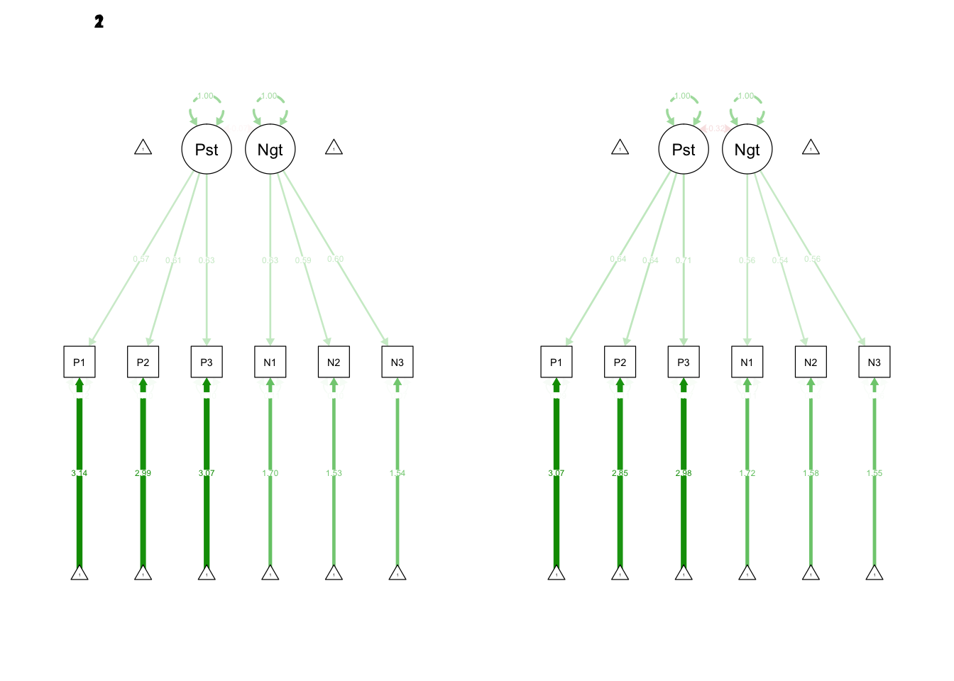
Need to put in labels to fix the different parameters across models
group2 <- 'Positive =~ c(L1,L1)*P1 + c(L2,L2)*P2 + c(L3,L3)*P3
Negative =~ N1 + N2 + N3

Positive ~~ 1*Positive
Negative ~~ 1*Negative

Positive ~~ Negative
'

fit.group.2 <- cfa(group2, data=group, std.lv=TRUE, group = "Grade")

summary(fit.group.2, standardized=TRUE, fit.measures=TRUE)
## lavaan (0.5-23.1097) converged normally after 52 iterations
##
## Number of observations per group
## 7th 380
## 8th 379
##
## Estimator ML
## Minimum Function Test Statistic 51.058
## Degrees of freedom 19
## P-value (Chi-square) 0.000
##
## Chi-square for each group:
##
## 7th 19.934
## 8th 31.124
##
## Model test baseline model:
##
## Minimum Function Test Statistic 3598.760
## Degrees of freedom 30
## P-value 0.000
##
## User model versus baseline model:
##
## Comparative Fit Index (CFI) 0.991
## Tucker-Lewis Index (TLI) 0.986
##
## Loglikelihood and Information Criteria:
##
## Loglikelihood user model (H0) -2904.111
## Loglikelihood unrestricted model (H1) -2878.582
##
## Number of free parameters 35
## Akaike (AIC) 5878.222
## Bayesian (BIC) 6040.342
## Sample-size adjusted Bayesian (BIC) 5929.203
##
## Root Mean Square Error of Approximation:
##
## RMSEA 0.067
## 90 Percent Confidence Interval 0.045 0.089
## P-value RMSEA <= 0.05 0.098
##
## Standardized Root Mean Square Residual:
##
## SRMR 0.048
##
## Parameter Estimates:
##
## Information Expected
## Standard Errors Standard
##
##
## Group 1 [7th]:
##
## Latent Variables:
## Estimate Std.Err z-value P(>|z|) Std.lv Std.all
## Positive =~
## P1 (L1) 0.607 0.020 30.548 0.000 0.607 0.871
## P2 (L2) 0.621 0.020 30.504 0.000 0.621 0.886
## P3 (L3) 0.674 0.021 32.232 0.000 0.674 0.906
## Negative =~
## N1 0.634 0.029 21.642 0.000 0.634 0.888
## N2 0.585 0.027 21.461 0.000 0.585 0.884
## N3 0.599 0.026 22.816 0.000 0.599 0.918
##
## Covariances:
## Estimate Std.Err z-value P(>|z|) Std.lv Std.all
## Positive ~~
## Negative -0.074 0.055 -1.343 0.179 -0.074 -0.074
##
## Intercepts:
## Estimate Std.Err z-value P(>|z|) Std.lv Std.all
## .P1 3.136 0.036 87.656 0.000 3.136 4.497
## .P2 2.991 0.036 83.103 0.000 2.991 4.263
## .P3 3.069 0.038 80.434 0.000 3.069 4.126
## .N1 1.701 0.037 46.473 0.000 1.701 2.384
## .N2 1.527 0.034 44.936 0.000 1.527 2.305
## .N3 1.545 0.033 46.185 0.000 1.545 2.369
## Positive 0.000 0.000 0.000
## Negative 0.000 0.000 0.000
##
## Variances:
## Estimate Std.Err z-value P(>|z|) Std.lv Std.all
## Positive 1.000 1.000 1.000
## Negative 1.000 1.000 1.000
## .P1 0.118 0.012 9.839 0.000 0.118 0.242
## .P2 0.106 0.012 9.121 0.000 0.106 0.216
## .P3 0.099 0.012 7.968 0.000 0.099 0.179
## .N1 0.107 0.012 9.215 0.000 0.107 0.211
## .N2 0.096 0.010 9.467 0.000 0.096 0.219
## .N3 0.067 0.009 7.308 0.000 0.067 0.157
##
##
## Group 2 [8th]:
##
## Latent Variables:
## Estimate Std.Err z-value P(>|z|) Std.lv Std.all
## Positive =~
## P1 (L1) 0.607 0.020 30.548 0.000 0.607 0.901
## P2 (L2) 0.621 0.020 30.504 0.000 0.621 0.888
## P3 (L3) 0.674 0.021 32.232 0.000 0.674 0.928
## Negative =~
## N1 0.559 0.027 20.740 0.000 0.559 0.864
## N2 0.542 0.024 22.303 0.000 0.542 0.905
## N3 0.563 0.025 22.922 0.000 0.563 0.920
##
## Covariances:
## Estimate Std.Err z-value P(>|z|) Std.lv Std.all
## Positive ~~
## Negative -0.308 0.050 -6.180 0.000 -0.308 -0.308
##
## Intercepts:
## Estimate Std.Err z-value P(>|z|) Std.lv Std.all
## .P1 3.073 0.035 88.799 0.000 3.073 4.561
## .P2 2.847 0.036 79.220 0.000 2.847 4.069
## .P3 2.979 0.037 79.802 0.000 2.979 4.099
## .N1 1.717 0.033 51.640 0.000 1.717 2.653
## .N2 1.580 0.031 51.345 0.000 1.580 2.637
## .N3 1.550 0.031 49.363 0.000 1.550 2.536
## Positive 0.000 0.000 0.000
## Negative 0.000 0.000 0.000
##
## Variances:
## Estimate Std.Err z-value P(>|z|) Std.lv Std.all
## Positive 1.000 1.000 1.000
## Negative 1.000 1.000 1.000
## .P1 0.085 0.009 9.240 0.000 0.085 0.188
## .P2 0.104 0.010 9.940 0.000 0.104 0.212
## .P3 0.074 0.010 7.434 0.000 0.074 0.140
## .N1 0.106 0.010 10.399 0.000 0.106 0.254
## .N2 0.065 0.008 8.288 0.000 0.065 0.181
## .N3 0.057 0.008 7.227 0.000 0.057 0.153We could now test whether constraining the groups makes the fit worse (similar to how we did it for measurement invariance)
anova(fit.group.1,fit.group.2)## Chi Square Difference Test
##
## Df AIC BIC Chisq Chisq diff Df diff Pr(>Chisq)
## fit.group.1 16 5879.3 6055.3 46.102
## fit.group.2 19 5878.2 6040.3 51.058 4.9557 3 0.1751What if you wanted to make everything the same for a particular type of parameter? Lavaan has an easier answer:
group3 <- 'Positive =~ P1 + P2 + P3
Negative =~ N1 + N2 + N3

Positive ~~ 1*Positive
Negative ~~ 1*Negative

Positive ~~ Negative
'

fit.group.3 <- cfa(group3, data=group, std.lv=TRUE, group = "Grade", group.equal = c("loadings", "intercepts"))

summary(fit.group.3, standardized=TRUE, fit.measures=TRUE)
## lavaan (0.5-23.1097) converged normally after 58 iterations
##
## Number of observations per group
## 7th 380
## 8th 379
##
## Estimator ML
## Minimum Function Test Statistic 64.155
## Degrees of freedom 26
## P-value (Chi-square) 0.000
##
## Chi-square for each group:
##
## 7th 26.771
## 8th 37.384
##
## Model test baseline model:
##
## Minimum Function Test Statistic 3598.760
## Degrees of freedom 30
## P-value 0.000
##
## User model versus baseline model:
##
## Comparative Fit Index (CFI) 0.989
## Tucker-Lewis Index (TLI) 0.988
##
## Loglikelihood and Information Criteria:
##
## Loglikelihood user model (H0) -2910.660
## Loglikelihood unrestricted model (H1) -2878.582
##
## Number of free parameters 28
## Akaike (AIC) 5877.319
## Bayesian (BIC) 6007.015
## Sample-size adjusted Bayesian (BIC) 5918.104
##
## Root Mean Square Error of Approximation:
##
## RMSEA 0.062
## 90 Percent Confidence Interval 0.043 0.082
## P-value RMSEA <= 0.05 0.137
##
## Standardized Root Mean Square Residual:
##
## SRMR 0.059
##
## Parameter Estimates:
##
## Information Expected
## Standard Errors Standard
##
##
## Group 1 [7th]:
##
## Latent Variables:
## Estimate Std.Err z-value P(>|z|) Std.lv Std.all
## Positive =~
## P1 (.p1.) 0.607 0.020 30.559 0.000 0.607 0.870
## P2 (.p2.) 0.624 0.020 30.563 0.000 0.624 0.886
## P3 (.p3.) 0.675 0.021 32.293 0.000 0.675 0.906
## Negative =~
## N1 (.p4.) 0.596 0.020 29.973 0.000 0.596 0.873
## N2 (.p5.) 0.564 0.018 31.005 0.000 0.564 0.875
## N3 (.p6.) 0.581 0.018 32.359 0.000 0.581 0.916
##
## Covariances:
## Estimate Std.Err z-value P(>|z|) Std.lv Std.all
## Positive ~~
## Negative -0.072 0.055 -1.305 0.192 -0.072 -0.072
##
## Intercepts:
## Estimate Std.Err z-value P(>|z|) Std.lv Std.all
## .P1 (.16.) 3.153 0.034 92.887 0.000 3.153 4.521
## .P2 (.17.) 2.966 0.035 85.406 0.000 2.966 4.211
## .P3 (.18.) 3.077 0.037 83.037 0.000 3.077 4.133
## .N1 (.19.) 1.697 0.033 50.786 0.000 1.697 2.485
## .N2 (.20.) 1.545 0.031 49.198 0.000 1.545 2.399
## .N3 (.21.) 1.535 0.032 48.359 0.000 1.535 2.420
## Positiv 0.000 0.000 0.000
## Negativ 0.000 0.000 0.000
##
## Variances:
## Estimate Std.Err z-value P(>|z|) Std.lv Std.all
## Positive 1.000 1.000 1.000
## Negative 1.000 1.000 1.000
## .P1 0.118 0.012 9.870 0.000 0.118 0.243
## .P2 0.107 0.012 9.109 0.000 0.107 0.215
## .P3 0.099 0.012 7.946 0.000 0.099 0.178
## .N1 0.111 0.011 9.751 0.000 0.111 0.237
## .N2 0.097 0.010 9.681 0.000 0.097 0.234
## .N3 0.065 0.009 7.382 0.000 0.065 0.162
##
##
## Group 2 [8th]:
##
## Latent Variables:
## Estimate Std.Err z-value P(>|z|) Std.lv Std.all
## Positive =~
## P1 (.p1.) 0.607 0.020 30.559 0.000 0.607 0.900
## P2 (.p2.) 0.624 0.020 30.563 0.000 0.624 0.888
## P3 (.p3.) 0.675 0.021 32.293 0.000 0.675 0.928
## Negative =~
## N1 (.p4.) 0.596 0.020 29.973 0.000 0.596 0.879
## N2 (.p5.) 0.564 0.018 31.005 0.000 0.564 0.911
## N3 (.p6.) 0.581 0.018 32.359 0.000 0.581 0.923
##
## Covariances:
## Estimate Std.Err z-value P(>|z|) Std.lv Std.all
## Positive ~~
## Negative -0.316 0.049 -6.434 0.000 -0.316 -0.316
##
## Intercepts:
## Estimate Std.Err z-value P(>|z|) Std.lv Std.all
## .P1 (.16.) 3.153 0.034 92.887 0.000 3.153 4.680
## .P2 (.17.) 2.966 0.035 85.406 0.000 2.966 4.222
## .P3 (.18.) 3.077 0.037 83.037 0.000 3.077 4.230
## .N1 (.19.) 1.697 0.033 50.786 0.000 1.697 2.502
## .N2 (.20.) 1.545 0.031 49.198 0.000 1.545 2.497
## .N3 (.21.) 1.535 0.032 48.359 0.000 1.535 2.440
## Positiv -0.153 0.076 -2.028 0.043 -0.153 -0.153
## Negativ 0.040 0.075 0.527 0.598 0.040 0.040
##
## Variances:
## Estimate Std.Err z-value P(>|z|) Std.lv Std.all
## Positive 1.000 1.000 1.000
## Negative 1.000 1.000 1.000
## .P1 0.086 0.009 9.277 0.000 0.086 0.189
## .P2 0.104 0.010 9.930 0.000 0.104 0.211
## .P3 0.074 0.010 7.418 0.000 0.074 0.139
## .N1 0.104 0.010 10.299 0.000 0.104 0.227
## .N2 0.065 0.008 8.576 0.000 0.065 0.170
## .N3 0.058 0.008 7.722 0.000 0.058 0.147What is nice is that the output will label what parameters are constrained. Go ahead and look at the lavaan tutorial for more (residual variances, latent means, etc)
7.11.1 measurement invariance revisited
Can you see how MI tests are just a special type of multiple group analysis? We could set up our data to have variables assessed at two different time points with the time demarcated by a group variable. The exact same findings from MI would be found with multiple group. It all depends on how you structure your data.
7.11.2 When to use
For Longitudinal models you are faced with a choice: do you want to use group status to predit your slope, for example, or do you want to use multiple groups. The short answer is that it does not matter! The semi-longer answer is that including group as a predictor is simple while multiple groups analyses are more complex but also more flexible. Using one or the other depends on what your theory about where the group differences occur. If they occur in only the regression relationshop indicating group mean differences then go with the easy option. If you think that the measurement model also may differ for your groups you have a more nuanced theory that necessiates multiple groups.
Demo.growth$group <- cut(Demo.growth$x1.c, breaks=c(-Inf, 0, Inf), labels=c("low", "high"))

model.7 <- '
  # intercept and slope with fixed coefficients
    i =~ 1*t1 + 1*t2 + 1*t3 + 1*t4
    s =~ 0*t1 + 1*t2 + 2*t3 + 3*t4
  # regressions
    i ~ group
    s ~ group
'
fit.7 <- growth(model.7, data = Demo.growth)
summary(fit.7)
## lavaan (0.5-23.1097) converged normally after 36 iterations
##
## Number of observations 400
##
## Estimator ML
## Minimum Function Test Statistic 8.925
## Degrees of freedom 7
## P-value (Chi-square) 0.258
##
## Parameter Estimates:
##
## Information Expected
## Standard Errors Standard
##
## Latent Variables:
## Estimate Std.Err z-value P(>|z|)
## i =~
## t1 1.000
## t2 1.000
## t3 1.000
## t4 1.000
## s =~
## t1 0.000
## t2 1.000
## t3 2.000
## t4 3.000
##
## Regressions:
## Estimate Std.Err z-value P(>|z|)
## i ~
## group 1.155 0.142 8.115 0.000
## s ~
## group 0.568 0.079 7.226 0.000
##
## Covariances:
## Estimate Std.Err z-value P(>|z|)
## .i ~~
## .s 0.454 0.061 7.389 0.000
##
## Intercepts:
## Estimate Std.Err z-value P(>|z|)
## .t1 0.000
## .t2 0.000
## .t3 0.000
## .t4 0.000
## .i -1.120 0.225 -4.972 0.000
## .s 0.153 0.124 1.227 0.220
##
## Variances:
## Estimate Std.Err z-value P(>|z|)
## .t1 0.593 0.085 6.950 0.000
## .t2 0.679 0.061 11.104 0.000
## .t3 0.632 0.072 8.811 0.000
## .t4 0.510 0.123 4.153 0.000
## .i 1.599 0.150 10.667 0.000
## .s 0.506 0.046 10.935 0.000model.8 <- '
# intercept and slope with fixed coefficients
i =~ 1*t1 + 1*t2 + 1*t3 + 1*t4
s =~ 0*t1 + 1*t2 + 2*t3 + 3*t4
'
fit.8 <- growth(model.8, data = Demo.growth, group = "group")
summary(fit.8)## lavaan (0.5-23.1097) converged normally after 41 iterations
##
## Number of observations per group
## low 199
## high 201
##
## Estimator ML
## Minimum Function Test Statistic 10.644
## Degrees of freedom 10
## P-value (Chi-square) 0.386
##
## Chi-square for each group:
##
## low 8.116
## high 2.528
##
## Parameter Estimates:
##
## Information Expected
## Standard Errors Standard
##
##
## Group 1 [low]:
##
## Latent Variables:
## Estimate Std.Err z-value P(>|z|)
## i =~
## t1 1.000
## t2 1.000
## t3 1.000
## t4 1.000
## s =~
## t1 0.000
## t2 1.000
## t3 2.000
## t4 3.000
##
## Covariances:
## Estimate Std.Err z-value P(>|z|)
## i ~~
## s 0.465 0.092 5.036 0.000
##
## Intercepts:
## Estimate Std.Err z-value P(>|z|)
## .t1 0.000
## .t2 0.000
## .t3 0.000
## .t4 0.000
## i 0.032 0.104 0.309 0.757
## s 0.722 0.058 12.495 0.000
##
## Variances:
## Estimate Std.Err z-value P(>|z|)
## .t1 0.519 0.118 4.417 0.000
## .t2 0.680 0.087 7.827 0.000
## .t3 0.635 0.103 6.190 0.000
## .t4 0.505 0.178 2.838 0.005
## i 1.754 0.224 7.824 0.000
## s 0.559 0.070 7.999 0.000
##
##
## Group 2 [high]:
##
## Latent Variables:
## Estimate Std.Err z-value P(>|z|)
## i =~
## t1 1.000
## t2 1.000
## t3 1.000
## t4 1.000
## s =~
## t1 0.000
## t2 1.000
## t3 2.000
## t4 3.000
##
## Covariances:
## Estimate Std.Err z-value P(>|z|)
## i ~~
## s 0.445 0.081 5.469 0.000
##
## Intercepts:
## Estimate Std.Err z-value P(>|z|)
## .t1 0.000
## .t2 0.000
## .t3 0.000
## .t4 0.000
## i 1.190 0.097 12.213 0.000
## s 1.288 0.053 24.175 0.000
##
## Variances:
## Estimate Std.Err z-value P(>|z|)
## .t1 0.671 0.124 5.419 0.000
## .t2 0.674 0.086 7.877 0.000
## .t3 0.628 0.100 6.263 0.000
## .t4 0.525 0.169 3.099 0.002
## i 1.446 0.200 7.224 0.000
## s 0.451 0.061 7.404 0.000Notice how the slope and the intercept are larger for the high group, suggesting a difference between groups.
model.9 <- '
  # intercept and slope with fixed coefficients
    i =~ 1*t1 + 1*t2 + 1*t3 + 1*t4
    s =~ 0*t1 + 1*t2 + 2*t3 + 3*t4

'
fit.9 <- growth(model.9, data = Demo.growth, group = "group", group.equal = "means")
summary(fit.9)
## lavaan (0.5-23.1097) converged normally after 46 iterations
##
## Number of observations per group
## low 199
## high 201
##
## Estimator ML
## Minimum Function Test Statistic 95.634
## Degrees of freedom 12
## P-value (Chi-square) 0.000
##
## Chi-square for each group:
##
## low 55.362
## high 40.272
##
## Parameter Estimates:
##
## Information Expected
## Standard Errors Standard
##
##
## Group 1 [low]:
##
## Latent Variables:
## Estimate Std.Err z-value P(>|z|)
## i =~
## t1 1.000
## t2 1.000
## t3 1.000
## t4 1.000
## s =~
## t1 0.000
## t2 1.000
## t3 2.000
## t4 3.000
##
## Covariances:
## Estimate Std.Err z-value P(>|z|)
## i ~~
## s 0.664 0.109 6.082 0.000
##
## Intercepts:
## Estimate Std.Err z-value P(>|z|)
## .t1 0.000
## .t2 0.000
## .t3 0.000
## .t4 0.000
## i (.20.) 0.665 0.077 8.684 0.000
## s (.21.) 1.036 0.042 24.903 0.000
##
## Variances:
## Estimate Std.Err z-value P(>|z|)
## .t1 0.526 0.118 4.442 0.000
## .t2 0.673 0.087 7.780 0.000
## .t3 0.641 0.104 6.174 0.000
## .t4 0.499 0.180 2.775 0.006
## i 2.152 0.263 8.189 0.000
## s 0.658 0.080 8.276 0.000
##
##
## Group 2 [high]:
##
## Latent Variables:
## Estimate Std.Err z-value P(>|z|)
## i =~
## t1 1.000
## t2 1.000
## t3 1.000
## t4 1.000
## s =~
## t1 0.000
## t2 1.000
## t3 2.000
## t4 3.000
##
## Covariances:
## Estimate Std.Err z-value P(>|z|)
## i ~~
## s 0.578 0.092 6.253 0.000
##
## Intercepts:
## Estimate Std.Err z-value P(>|z|)
## .t1 0.000
## .t2 0.000
## .t3 0.000
## .t4 0.000
## i (.20.) 0.665 0.077 8.684 0.000
## s (.21.) 1.036 0.042 24.903 0.000
##
## Variances:
## Estimate Std.Err z-value P(>|z|)
## .t1 0.670 0.124 5.393 0.000
## .t2 0.675 0.086 7.862 0.000
## .t3 0.626 0.101 6.205 0.000
## .t4 0.527 0.171 3.081 0.002
## i 1.722 0.227 7.599 0.000
## s 0.514 0.067 7.685 0.000Does constraining the latent means lead to a worse fit?
anova(fit.8, fit.9)## Chi Square Difference Test
##
## Df AIC BIC Chisq Chisq diff Df diff Pr(>Chisq)
## fit.8 10 5458.5 5530.3 10.644
## fit.9 12 5539.5 5603.3 95.634 84.99 2 < 2.2e-16 ***
## ---
## Signif. codes: 0 '***' 0.001 '**' 0.01 '*' 0.05 '.' 0.1 ' ' 1testing just the slope difference without constraining anything else.
model.10 <- '
  # intercept and slope with fixed coefficients
    i =~ 1*t1 + 1*t2 + 1*t3 + 1*t4
    s =~ 0*t1 + 1*t2 + 2*t3 + 3*t4

s ~  c(m1, m1)*1

'
fit.10 <- growth(model.10, data = Demo.growth, group = "group")
summary(fit.10)
## lavaan (0.5-23.1097) converged normally after 44 iterations
##
## Number of observations per group
## low 199
## high 201
##
## Estimator ML
## Minimum Function Test Statistic 59.434
## Degrees of freedom 11
## P-value (Chi-square) 0.000
##
## Chi-square for each group:
##
## low 34.932
## high 24.502
##
## Parameter Estimates:
##
## Information Expected
## Standard Errors Standard
##
##
## Group 1 [low]:
##
## Latent Variables:
## Estimate Std.Err z-value P(>|z|)
## i =~
## t1 1.000
## t2 1.000
## t3 1.000
## t4 1.000
## s =~
## t1 0.000
## t2 1.000
## t3 2.000
## t4 3.000
##
## Covariances:
## Estimate Std.Err z-value P(>|z|)
## i ~~
## s 0.505 0.099 5.110 0.000
##
## Intercepts:
## Estimate Std.Err z-value P(>|z|)
## s (m1) 1.032 0.042 24.792 0.000
## .t1 0.000
## .t2 0.000
## .t3 0.000
## .t4 0.000
## i 0.174 0.102 1.706 0.088
##
## Variances:
## Estimate Std.Err z-value P(>|z|)
## .t1 0.504 0.118 4.279 0.000
## .t2 0.686 0.088 7.835 0.000
## .t3 0.641 0.105 6.125 0.000
## .t4 0.495 0.184 2.692 0.007
## i 1.781 0.226 7.871 0.000
## s 0.657 0.079 8.295 0.000
##
##
## Group 2 [high]:
##
## Latent Variables:
## Estimate Std.Err z-value P(>|z|)
## i =~
## t1 1.000
## t2 1.000
## t3 1.000
## t4 1.000
## s =~
## t1 0.000
## t2 1.000
## t3 2.000
## t4 3.000
##
## Covariances:
## Estimate Std.Err z-value P(>|z|)
## i ~~
## s 0.476 0.086 5.541 0.000
##
## Intercepts:
## Estimate Std.Err z-value P(>|z|)
## s (m1) 1.032 0.042 24.792 0.000
## .t1 0.000
## .t2 0.000
## .t3 0.000
## .t4 0.000
## i 1.077 0.096 11.175 0.000
##
## Variances:
## Estimate Std.Err z-value P(>|z|)
## .t1 0.677 0.125 5.416 0.000
## .t2 0.672 0.086 7.851 0.000
## .t3 0.623 0.101 6.161 0.000
## .t4 0.535 0.174 3.070 0.002
## i 1.457 0.202 7.228 0.000
## s 0.515 0.067 7.671 0.000anova(fit.8, fit.10)## Chi Square Difference Test
##
## Df AIC BIC Chisq Chisq diff Df diff Pr(>Chisq)
## fit.8 10 5458.5 5530.3 10.644
## fit.10 11 5505.3 5573.1 59.434 48.79 1 2.849e-12 ***
## ---
## Signif. codes: 0 '***' 0.001 '**' 0.01 '*' 0.05 '.' 0.1 ' ' 17.12 Missing data
7.12.1 Planned missing data
7.13 Power
7.14 Now you try
Fit a measurement model to your constructs at one time point. Try out the different types of scaling discussed in class. What changes what stays the same?
- What do the fit statistics say about your latent variable? Good/bad? Is your latent variable Just identified/saturdated, under identified or over identified?
Fit a longitudinal CFA model where you a) first correlate your latent factors across time and then b) a second model that predicts later times by a prevous time (ie auto regressive; t1 -> t2 -> t3). What are your conclusions? How does one differ from the other?
Fit a longitdinal growth model in SEM and in HLM. Compare and contrast the differences.
Constrain the residual variances to be equal. Does this change the fit of your model?
Contrain your slope to be fixed, not random. How does this change your model?
Change the time metric in your SEM growth model. How does that change your estimates? Does it change your fit statistics?
Try a different type of estimation (see lavaan tutorial for details). How does that change your model?
Provide semplots for each of the models.
—-NEW QUESTIONS—-
Test measurement invariance across time for your construct. Can you run growth models? If there is evidence of non-invariance, what seems to be the problem?
Fit a second order growth model. Compare and contrast the estimates with the normal latent growth model.
Fit a series of multiple group models. Constrain some parameters and compare the fit.